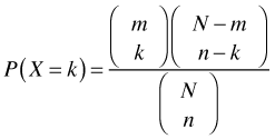
The hypergeometric model is the finite-population, sampling without replacement version of the binomial model. Whereas in the binomial model the probability of a success is constant from trial to trial, in the hypergeometric model the probability changes as selections are made. The standard illustration of a hypergeometric model is choosing colored balls from an urn. Suppose there are N balls in an urn of which m of them are red and the rest are black. The probability of drawing X = k red balls in a sample of size n balls is the following.

The first term in the numerator is the number of ways of choosing k red balls, the second term is the number of ways of choosing n – k black balls, and the denominator is the number of different samples of n balls. The mean and variance of the hypergeometric distribution are the following.

We can apply this to survival analysis as follows. For simplicity suppose there are just two groups. At failure time j there are a total of Oj failures in a risk set of Nj individuals of which n1j of the individuals are from group 1. The probability of observing k failures in group 1 is the hypergeometric distribution (assuming the same failure rate in both groups).
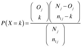
The log-rank test resembles the Pearson Χ2 test in its construction. At each failure time we obtain the expected number of deaths under a hypergeometric model for the current risk set assuming that there is a common failure rate in all the groups. We then subtract the expected number of deaths from the observed number of deaths in group 1. This is repeated at each failure time and the differences are summed. Treating the outcomes at each failure time as independent, the variance of the sum is just the sum of the hypergeometric variances at each event time. We divide the the summed differences by the square root of the variance of this sum under the hypergeometric model to obtain the test statistic of the log-rank test. When squared this test statistic has a chi-squared distribution.
In variations of this test the failure times are weighted differently in order to emphasize early events or late events. As an illustration when there are just two groups the log-rank test takes the following form.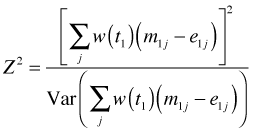
Here mij and eij are the observed and expected deaths for group i at failure time j. One version of the test (variously called the generalized Wilcoxon or Gehan-Wilcoxon or just the Gehan test) uses the number at risk in the group as the weight, a choice that tends to reward early survival over later survival. The log-rank test proper uses equally weighted observations which weights later survival more than the Gehan test does. The log-rank test is purely a test of significance and cannot be used to estimate the magnitude of the differences between groups.
One of the goals in the regression modeling of survival data is to obtain estimates of the survivor function after adjusting for measured covariates, something that is not possible with the Kaplan-Meier estimator. There are two standard approaches to regression analysis of survival data.
In addition we have the choice of a semi-parametric or a parametric model. Parametric models can be either proportional hazards or accelerated failure time models. The most popular semiparametric model is a proportional hazards model called Cox regression.
The Cox proportional hazards regression model is also called the Cox model, Cox regression, or just proportional hazards regression (although the latter is really a misnomer). It is extremely popular in medical fields where it is often the only kind of model that is considered. It is considered a semi-parametric model for reasons explained below. In Cox regression we model the hazard function as follows.

This is a model that is linear in the log hazard.

The hazard in Cox regression is the product of two terms.
 contains the linear predictor and multiplies the baseline hazard. Notice that this term does not involve t. The assumption being made is that the individual predictors, xi, are time-invariant.
There is a model called the extended Cox model that does allow covariates to be time-dependent.
The Cox model is called semi-parametric because the hazard function is not fully specified.
The regression coefficients of the Cox model are estimated by maximizing a quantity known as the partial likelihood (rather than a full likelihood). Recall that the likelihood is just the probability of obtaining the data that were obtained. In a partial likelihood for survival data rather than specifying P(data), we instead construct an expression for P(those who fail). Individuals who were censored do not contribute individual terms to the partial likelihood. Thus the likelihood takes the form
![]()
in which there are k failure times. At each failure time the censored individuals do contribute to the risk set and are used in calculating the individual terms of the likelihood.
Formally the Cox partial likelihood is constructed as follows. Let ![]() be the observation times for the n observations in the study and let
be the observation times for the n observations in the study and let ![]() be indicators of the event at those times, i.e.,
be indicators of the event at those times, i.e.,

Using the Cox model for the hazard, the hazard for individual i is just

Now form the following ratio.
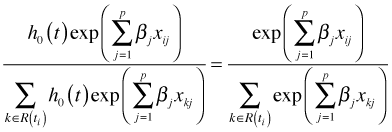
In the denominator we are summing the hazards for all individual still alive at time ti, i.e., members of the risk set R(ti). Notice that the baseline hazard ![]() cancels and does not appear in the final expression. The Cox partial likelihood is the product of all such terms.
cancels and does not appear in the final expression. The Cox partial likelihood is the product of all such terms.
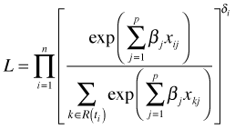
The use of δi as an exponent is just a convenient way of including all observations in the likelihood without having to single out the failure times. Observations that are censored have δi = 0 and hence contribute nothing to the likelihood (their contribution to the product is one).
In logistic regression the focus is on odds ratios. A similar quantity, the hazard ratio, plays a role in Cox regression. To construct the hazard ratio we just take the ratio of the hazards of two individuals who have different values of the covariates, x.

Now suppose

but for all other values of x, x = x*. Then we have ![]() for two individuals that differ only in their treatment. The hazard ratio in this instance tells us by what amount the hazard is multiplied for individuals in the treatment group relative to the control group while holding everything else constant.
for two individuals that differ only in their treatment. The hazard ratio in this instance tells us by what amount the hazard is multiplied for individuals in the treatment group relative to the control group while holding everything else constant.
Notice that because the baseline hazards cancel, the hazard ratio is constant with respect to time. This is the essence of the proportional hazards assumption. We'll discuss how one might go about testing this assumption in lecture 29, but what should one do if the assumption appears to be violated?
In parametric survival models an explicit probability model is chosen for the survival time distribution / hazard function. By choosing a probability model one also automatically chooses either a proportional hazards or an accelerated failure time model. Except for the Weibull (exponential) distributions, only one of these choices is possible with a given probability model. The disadvantages of the parametric approach are the following.
The advantages of the parametric approach are the following.
Let f(t) denote the probability density for the survival distribution. Table 4 summarizes how different kinds of censored observations contribute to the parametric likelihood of failure times. Note: F(0) = 0.
| Type | Event | Contribution to the likelihood |
|---|---|---|
| uncensored | T = 2 |
|
| right censored | T > 2 |
|
| left censored | T ≤ 2 |
|
| interval censored | 2 < T ≤ 3 |
While there are many potential probability models for survival distributions, the Weibull is the most commonly used and perhaps the most flexible. The Weibull survivor and hazard functions are shown below.

Here p = shape parameter and λ (typically its log) is modeled in terms of explanatory variables. The exponential distribution is a special case of the Weibull (p = 1).
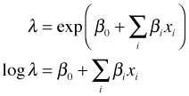
The Weibull distribution yields both a proportional hazards model and an accelerated failure time model depending on how things are parameterized. Having chosen one of the parameterizations it is possible to obtain the corresponding estimates for the other parameterization as Table 5 explains.
| Proportional hazards | Accelerated failure time |
|---|---|
 |
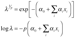 |
From Table 5 we see that we can switch between the parameterizations using the identity ![]() . Thus when βj < 0 in the proportional hazards parameterization (meaning the hazard is decreased by increasing the value of the predictor), it follows that αj > 0 in the accelerated failure time parameterization (meaning survival time is extended).
. Thus when βj < 0 in the proportional hazards parameterization (meaning the hazard is decreased by increasing the value of the predictor), it follows that αj > 0 in the accelerated failure time parameterization (meaning survival time is extended).
An alternative approach to interval censored data is to use what's known as discrete time survival analysis. Discrete time survival analysis uses binary logistic regression with dummy variables to indicate the different survival intervals. See Singer & Willett (2003), chapters 10–12, or Kleinbaum & Klein (2005), pp. 290–292, for more details.
| Jack Weiss Phone: (919) 962-5930 E-Mail: jack_weiss@unc.edu Address: Curriculum for the Environment and Ecology, Box 3275, University of North Carolina, Chapel Hill, 27599 Copyright © 2012 Last Revised--March 24, 2012 URL: https://sakai.unc.edu/access/content/group/2842013b-58f5-4453-aa8d-3e01bacbfc3d/public/Ecol562_Spring2012/docs/lectures/lecture28.htm |