Lecture 18—Monday, February 20, 2012

Topics

• Overview of the problem of observational heterogeneity
• Approaches for dealing with observational heterogeneity
  • Common pooling model
  • Fixed effects approach to dealing with observational heterogeneity
  • Random effects approach to dealing with observational heterogeneity

Overview

Observational heterogeneity occurs when some observations resemble others purely because of the way the data were collected.

• Suppose we have a random sample of individuals that we then follow over time obtaining multiple measurements from each individual. This is the classic repeated measures design. The sampling scheme has induced a structure in the data set. We expect that the different measurements coming from the same individual to be more similar to each other than to observations coming from different individuals. The coral core data we examined on Friday are data of this type.
• Suppose in an agricultural experiment we choose a number of different fields to which we randomly assign one of two fertilizer applications (I or II). Each individual field is then divided into four parts and four different crops (A, B, C, or D) are randomly assigned to the four quarters. Thus we have two "treatments", type of crop and type of fertilizer, applied to different sized units. The crop treatment is applied to quarters within a field while the fertilizer treatment is applied to fields (so that all the quarters in that field automatically get the same fertilizer treatment). Quarters are replicates of the crop treatment while fields are replicates of the fertilizer treatment. This is the classic split plot design in which we have different "sized" experimental units one of which is nested inside the other.

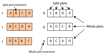
Fig. 1  Split plot design

Any time we have a lack of equivalence between the observational or experimental units used in a study, we have observational heterogeneity. Last week we discussed one specific approach for dealing with such heterogeneity—generalized least squares (GLS). We focused on the specific case of repeated measures data in which there is a long time series of data, but generalized least squares can be used any time data are organized in a hierarchical fashion. Unfortunately generalized least squares has some limitations.

• Because it generalizes ordinary least squares it is largely restricted to situations in which a normal distribution makes sense as a probability model for the response.
• Generalized least squares requires that we have a specific model in mind for the variances and covariances of our observations. With temporal data there some obvious choices which is why we focused on such data in our discussion of GLS. For other kinds of data the choice is not so obvious.

Today we discuss a second approach for dealing with observational heterogeneity in regression models—introducing random effects to produce what's called a mixed effects model. Mixed effects models are an omnibus way to account for observational heterogeneity. To set up a mixed model we just need to know how the data are structured, i.e., be able to identify the different sized units in the analysis. We don't actually have to understand the precise nature of the relationships (correlations) of the observations that make up the different sized units. Thus mixed effects models are a convenient way of addressing data structure especially in situations where the structure is a nuisance and is of little interest to us by itself. On the other hand if we fit a mixed effects model to temporal data it may still be necessary to account for lingering residual temporal correlation.

Approaches for dealing with observational heterogeneity

As an illustration of these basic ideas we return to the coral core data set we analyzed using generalized least squares last time. The basic goal was to model how coral extension rates (the widths of annual rings in coral cores) vary over time. The question of interest is whether extension rates have shown a linear trend over time that depends upon the location of the coral colony in the reef complex (nearshore, forereef, and backreef locations). We assume that extension rates are normally distributed with a mean that may be changing with time. Thus our basic assumption is where i denotes a coral core and j denotes an individual observation (annual ring) from that coral core.

Common pooling model

In the common pooling model we ignore the structure of the data entirely. We treat all of the observations as coming from a single population from which we've drawn a single random sample. For the coral core data set we would start by assuming that the mean is a linear function of calendar year.

where again i = core and j = individual observation from that core. The problem with the common pooling model is that it is almost certainly false. The errors are not independent as we saw last time. By ignoring data structure and treating the individual rings as being a random sample from the population of coral core annual rings we are guilty of pseudo-replication, claiming that we have an effective sample size that is much larger than the one we really have.

Fixed effects approach to dealing with observational heterogeneity

In the fixed effects approach to structured data, we include the structural variable as a predictor in the model. In the current example that translates into specifying dummy variables for individual cores and including them as additive terms and as interaction terms with year. This yields a separate intercept and slope for each core.

where g is the number of cores. As before, . The parameters β₀ and β₁ are the intercept and slope for core 1. β_i and γ_i are the deviations that the intercept and slope of core i exhibit from the intercept and slope of core 1. This single model is comparable to fitting separate regression models to each core except that when we do it using dummy variables in a single regression model we use all of the data to estimate the residual variance σ².

Although this approach gets the structure of the data set correct, something that was ignored in the common pooling model, it has other problems.

1. This model has the potential of severely overfitting the data. For instance, cores with only two observations (there are none in this data set) are fit perfectly.
2. We end up estimating a lot of different parameters, the individual core intercepts and slopes, that we really don't care about.
3. The model hampers our ability to test the hypothesis of interest, namely that the trend over time varies by reef type.
   1. We can't included reef type in this model because reef type is completely collinear with core. We can estimate a fixed effects model with reef type alone, or core alone, but not with both in the same model.
   2. If we fit a model with reef type alone or a model with core alone, the model with cores will certainly fit the data better than a model with just reef type. If we're lucky (as we were in lecture 17), the core model might not be a significant improvement over the reef type model and so we can argue that the reef type model is the more parsimonious one. This rarely occurs in practice.

Even though in lecture 17 we were able to simplify the separate slopes and intercepts model so that we needed to estimate only three slopes, one for each reef type, we were still left with estimating separate intercepts for each core. If there had been more cores used in the analysis it is unlikely we would have been able to make even this simplification. Fitting separate models to individual natural groups will nearly always provide a significantly better fit to data than will any simpler model that we can construct. The basic problem with the fixed effects approach is that it typically leads to overfitting the data.

Random effects approach to dealing with observational heterogeneity

The random effects analog of the separate slopes and intercepts regression model is the random slopes and intercepts model.

with . In this model β₀ and β₁ represent the population-average coefficients while and are the deviations from this population average for coral core i. β₀ and β₁ can also be interpreted as the regression coefficients for a typical core, i.e., one corresponding to the middle of the distribution of random effects. The intercept for core i is and the slope is . Thus the random slopes and intercepts formulation of this model is also the following.

What makes this model different from the fixed effects model is that and are not directly estimated but instead are assumed to be drawn from a multivariate normal distribution.

The diagonal entries of the multivariate normal covariance matrix are the individual variances of the intercept and slope random effects and the off-diagonal entry is their covariance. Because the correlation coefficient is defined by , an equivalent way of writing this distribution (and the one used by R) is the following.

Rather than estimate the individual and we instead estimate the parameters of the covariance matrix of the multivariate normal distribution: ρ, τ₀, and τ₁.

Course Home Page