Assignment 9—Solution

Question 1

My intention was that you just fit the six models treating beetle richness and relief as predictors in an additive model. The models in question are the following.

Question 2

Models mod1, mod2, mod3, and mod4 can be compared directly using log-likelihood and AIC. Models mod5 and mod6 involve a transformed response variable and therefore require some manipulation in order to compare them with the untransformed response models. The functions for this purpose were presented in lecture 20.

I obtain the log-likelihoods and AICs and assemble the results in a table.

The lognormal and negative binomial (NB-2) models are essentially tied, although technically the lognormal model has a slighlty lower AIC. At this point either model could be chosen. I would probably choose the negative binomial model only because it is a discrete probability model and makes it easier to interpret the response variable, which is a discrete count.

Variations on this answer

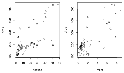
Many people considered transformations of the predictor. I didn't expect you to explore this possibility but it is certainly a legitimate thing to pursue. There is no theory to motivate the choice here. If we carry out a preliminary plot of the response variable versus each predictor separately both plots reveal what appear to be linear relationships (Fig. 1).

Fig. 1   Scatter plots of bird richness versus beetle richness and relief

A plot of the residuals of the lognormal or NB-2 models versus the predictors doesn't reveal anything especially unusual (Fig. 2).

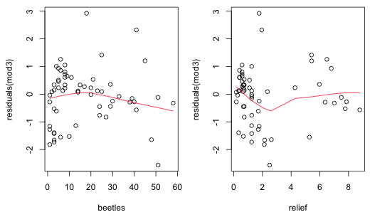
Fig. 2   Plot of residuals from negative binomial regression model (mod3) versus beetle richness and relief with a lowess curve superimposed.

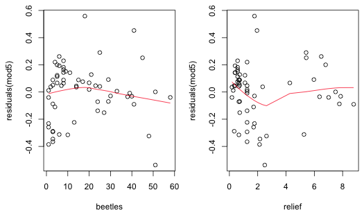
Fig. 3   Plot of residuals from a lognormal regression model (mod5) versus beetle richness and relief with a lowess curve superimposed.

None the less it turns out that if you include log(beetles) as a predictor you do get a better model in terms of AIC.

Once again the lognormal and negative binomial (NB-2) models are extremely competititve with the lognormal model ranking slightly ahead of the negative binomial. A residual plot does show a slight improvement.

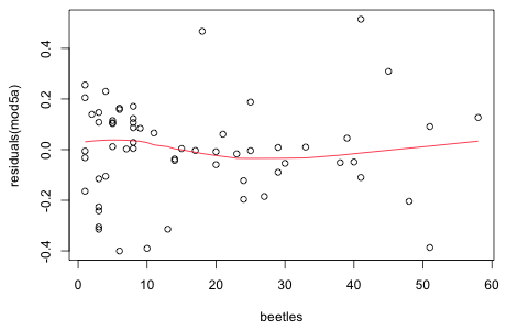
Fig. 4   Plot of residuals from a lognormal regression model with log(beetles) as a predictor (mod5a) versus beetle richness with a lowess curve superimposed.

Given that log-transforming the predictor does permit interpreting the bird-beetle relationship as a power law relationship one could argue that log-transforming beetles yields a model that is easier to interpret.

Question 3

Negative binomial model with beetles and relief as predictors

The fitted model is

Exponentiating both sides yields the following.

So beetle richness has a multiplicative effect on the mean. If beetle richness is increased by one unit we find

Raising beetle richness by one unit multiplies the mean by exp(β₁). Similarly increasing relief by one unit multiplies the mean by the factor exp(β₂).

So a one unit change in beetle richness leads to multiplying the mean by 1.013747, which is roughly a 1.4% increase in the mean. A one unit change in relief leads to multiplying the mean by 1.1, which is a 10% increase in the mean.

Negative binomial model with log(beetles) and relief as predictors

The fitted model is

The interpretation for a change in relief is the same as was described above for the previous model. With log predictors the proper way to think of effects is multiplicatively. Thus rather than adding one unit to beetle richness, we can think in terms of, say, a 1% change in beetle richness. To obtain a 1% change we multiply beetles by 1.01.

Subtracting the log old mean from the log new mean yields the following.

So a 1% change in beetle richness multiplies bird richness by = 1.00192, i.e., a .19% increase in the mean.

We can obtain a simpler interpretation of the effect as follows. The binomial series, a generalization of the binomial theorem, is given as follows.

for Δx small. Therefore we have

So a 1% increase in x leads to a β₁% increase in the mean, which again is approximately a .19% increase for a 1% increase in beetle richness.

Lognormal models

The fitted model with beetles and relief as predictors is

As was discussed in lecture 21, the mean of a log is not the same as the log of a mean. If we exponentiate the lefthand side we don't get the mean of the lognormal distribution. Instead we get the median. Thus the same interpretations described above for the negative binomial model apply to the lognormal except we apply it to the median rather than the mean. Thus a one unit change in beetles multiplies the median by exp(b1) while a one unit change in relief multiplies the median by exp(b2).

The fitted model with log(beetles) and relief as predicts is the following.

Now a 1% increase in beetles leads to a β₁% increase in the median, an approximately .19% increase.

Question 4

I plot the mean from the negative binomial model, mod3, but all of the predicted surfaces look about the same. To plot the regression surface we need to determine the range of the data and plot the surface only over that range.

I create a grid of values over this range, construct a function that defines the regression surface, and then evaluate the function over this grid.

The persp function requires that the z values be organized in a matrix that has the same dimensions as the grid over which we'll plot.

I play with the angle settings to get a surface in the most useful orientation.

To plot the points we need model predictions at each of the observed values. The trans3d function converts the 3-dimensional coordinates into the projected two-dimensional coordinates for plotting.

I use segments to draw the line segments and points to draw the points. For the colors I test if the observed points lie above the surface, convert the result to a number (0 for FALSE, 1 for TRUE), and 1 to the result so that we obtain 1 or 2. I then use this to select the first or second component of my color vector, c(4,2).

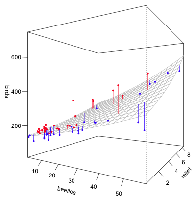
Fig. 5   Plot of the regression surface of the negative binomial regression model (mod3).

Question 5

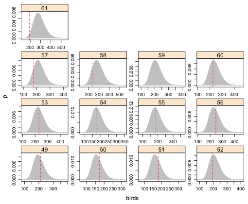
The code from lecture 20 can be used almost as is. The conditioning variable is "group" and there are 61 observations. I arrange the graph in a 4 x 4 layout. The code below graphically examines the fit of the negative binomial model mod3.

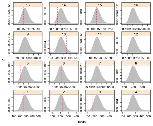
Fig. 6   (a) Predicted negative binomial distributions with observed bird richness values superimposed. Grid cells 1–16.

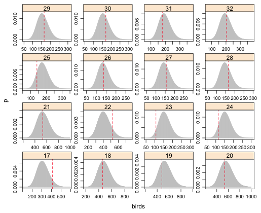
Fig. 6   (b) Predicted negative binomial distributions with observed bird richness values superimposed. Grid cells 17–32.

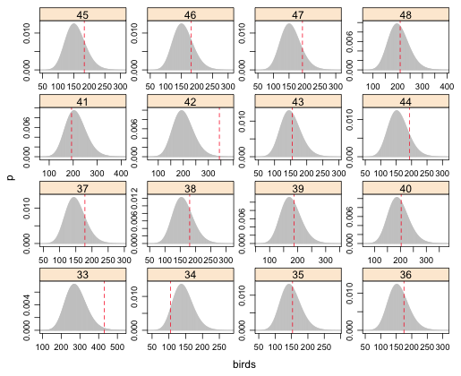
Fig. 6   (c) Predicted negative binomial distributions with observed bird richness values superimposed. Grid cells 33–48.

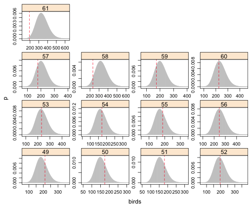
Fig. 6   (d) Predicted negative binomial distributions with observed bird richness values superimposed. Grid cells 49–61.

From the graphs the obvious instances of lack of fit are grid cells 61, 33, and perhaps 23.

Analytical test

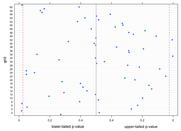
I calculate upper and lower p-values for each observed value and count the number that are less than .025, (two-tailed test). I display the results in a graph.

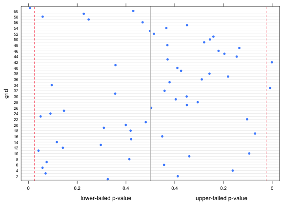
Fig. 7   Lower and upper-tailed p-values for the observed bird richness values with respect to negative binomial regression model. Vertical lines represent lower and upper 2.5% quantiles.

Three observations out of 61 are clear outliers, which is less than 5% of the values, not more than we'd expect to obtain by chance.

Fit of lognormal model

To examine the fit of the lognormal model the same code will work except we need to us the dlnorm function rather than dnbinom. The arguments of dlnorm are meanlog, which we obtain as the fitted values of our model, and sdlog, which is the square root of the average of the squared residuals. In the graph I display the fit for only the first 16 grid cells for the lognormal model with log(beetles) and relief as predictors.

Fig. 7   Predicted lognormal distributions with observed bird richness values superimposed. Grid cells 49–61.

Fig. 9   Lower and upper-tailed p-values for the observed bird richness values with respect to a lognormal regression model with log(beetles) and relief as predictors. Vertical lines represent lower and upper 2.5% quantiles.

Five observations out of 61 are clear outliers, which is about 8% of the values. This is more than we'd expect to obtain by chance. So, although the lognormal model with log(beetles) and relief as predictors had a lower AIC than a negative binomial model with beetles and relief as predictors, the lognormal model appears to fit fewer grid cells.

Question 6

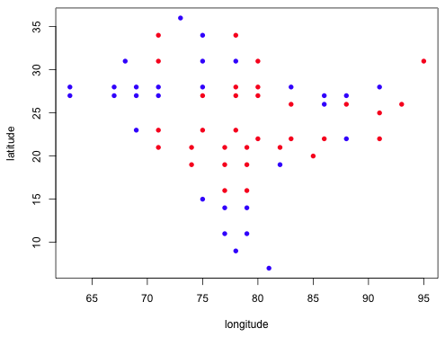
Fig. 10   Plot of negative binomial residuals by sign (red = positive, blue = negative) by their geographic location

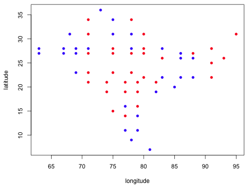
Fig. 11   Plot of lognormal residuals by sign (red = positive, blue = negative) by their geographic location

Both models show that the residuals of the same sign are clustered geographically suggesting that the model residuals are not independent. This is a violation of one of the assumptions of the regression model. We can formally assess this correlation analytically by carrying out a Mantel test. A Mantel test calculates the correlation between the geographic distances of points with the distance in the value of their residuals. It assesses the significance of the correlation using a randomization test. Residuals are randomly assigned to geographic location and the correlation of the randomized residuals is used to construct a null distribution for the statistic.

Call:
mantel(xdis = dist1, ydis = dist2)

Mantel statistic r: 0.335
      Significance: 0.001

Empirical upper confidence limits of r:
   90%    95%  97.5%    99%
0.0765 0.1040 0.1199 0.1418

Based on 999 permutations

Call:
mantel(xdis = dist1, ydis = dist2a)

Mantel statistic r: 0.2382
      Significance: 0.001

Empirical upper confidence limits of r:
  90%   95% 97.5%   99%
0.080 0.101 0.122 0.143

Based on 999 permutations

Both tests indicate a significant degree of spatial correlation in the residuals. A solution would be to add a spatial correlation structure for the residuals. This is easy to do for the lognormal model using generalized least squares (gls function of the nlme package), but more difficult for the negative binomial model. At this point I would switch exclusively to the lognormal model and adding a model for the residual correlation component using the gls function from the nlme package.

Course Home Page