Assignment 8—Solution
Question 1
stirrett <- read.delim('ecol 563/Stirrett.txt')
stirrett
Count Trt1 Trt2 Trt3 Trt4
1 0 19 24 43 47
2 1 12 16 35 23
3 2 18 16 17 27
4 3 18 18 11 9
5 4 11 15 5 7
6 5 12 9 4 3
7 6 7 6 1 1
8 7 8 5 2 1
9 8 4 3 2 0
10 9 4 4 0 0
11 10 1 3 0 1
12 11 0 0 0 1
13 12 1 1 0 0
14 13 1 0 0 0
15 15 1 0 0 0
16 17 1 0 0 0
17 19 1 0 0 0
18 26 1 0 0 0
These are the tabulated data. I begin by generating the raw data. I do this separately by treatment, using the rep function to repeat the values in the Count column the number of times indicated in each of the treatment columns.
trt1 <- rep(stirrett$Count, stirrett$Trt1)
trt2 <- rep(stirrett$Count, stirrett$Trt2)
trt3 <- rep(stirrett$Count, stirrett$Trt3)
trt4 <- rep(stirrett$Count, stirrett$Trt4)
Next we concatenate the counts contained in these three treatment vectors and add a second column that records the treatment to which they correspond.
borer <- data.frame(count = c(trt1, trt2, trt3, trt4), treatment = rep(1:4, c(length(trt1), length(trt2), length(trt3), length(trt4))))
dim(borer)
[1] 480 2
We're told that the four treatments are connected in a special way. They correspond to combining the levels of two binary factor variables in all possible ways. The correspondence is detailed in Table 1 where we see that treatments 3 and 4 received an early application of fungal spores, while treatments 2 and 4 received a late application of fungal spores. I add these two factors as two additional columns of the data frame.
borer$early <- factor(ifelse(borer$treatment %in% c(3,4), 'present', 'absent'))
borer$late <- factor(ifelse(borer$treatment %in% c(2,4), 'present', 'absent'))
When treatments are created by combining factors it is always advantageous to analyze the experiment as a factorial design in this case with two factors rather than as a one-way design with a single treatment. The two-factor interaction model yields a model that is identical to the one-way design. It's just parameterized differently. If the two-factor interaction is significant then nothing has been accomplished by analyzing things as a factorial design. If the interaction is not significant then we can then proceed to simplify the model and perhaps end up with a much simpler interpretation of the effect of treatment. I fit a two-factor interaction model assuming a negative binomial distribution for the response. I use the anova function to obtain sequential likelihood ratio tests.
library(MASS)
out.NB1 <- glm.nb(count~early*late, data=borer)
anova(out.NB1)
Analysis of Deviance Table
Model: Negative Binomial(1.4714), link: log
Response: count
Terms added sequentially (first to last)
Df Deviance Resid. Df Resid. Dev Pr(>Chi)
NULL 479 623.56
early 1 81.157 478 542.41 <2e-16 ***
late 1 1.927 477 540.48 0.1651
early:late 1 1.738 476 538.74 0.1874
---
Signif. codes: 0 ‘***’ 0.001 ‘**’ 0.01 ‘*’ 0.05 ‘.’ 0.1 ‘ ’ 1
Warning message:
In anova.negbin(out.NB1) : tests made without re-estimating 'theta'
Reading from the bottom of the table up we see that the two-factor interaction between early and late is not significant. Furthermore we also see the late main effect is also not significant given that the early effect is already in the model. The early effect is highly significant. I refit the model with just an early effect.
out.NB2 <- glm.nb(count~early, data=borer)
Question 2
To carry out the goodness of fit tests we need to work with the tabulated data. As we've seen, not all of the count categories are shown in the table. Intermediate categories that were not recorded for any of the four treatments are not included. For the goodness of fit test we need to include these missing categories and assign them a frequency of zero. Following the hint for this problem we can carry this out by creating a dummy data frame with just the full set of count categories and then merge this data frame with the tabulated data.
junk <- data.frame(Count=0:26)
borer.table <- merge(stirrett, junk, all=T)
borer.table
Count Trt1 Trt2 Trt3 Trt4
1 0 19 24 43 47
2 1 12 16 35 23
3 2 18 16 17 27
4 3 18 18 11 9
5 4 11 15 5 7
6 5 12 9 4 3
7 6 7 6 1 1
8 7 8 5 2 1
9 8 4 3 2 0
10 9 4 4 0 0
11 10 1 3 0 1
12 11 0 0 0 1
13 12 1 1 0 0
14 13 1 0 0 0
15 14 NA NA NA NA
16 15 1 0 0 0
17 16 NA NA NA NA
18 17 1 0 0 0
19 18 NA NA NA NA
20 19 1 0 0 0
21 20 NA NA NA NA
22 21 NA NA NA NA
23 22 NA NA NA NA
24 23 NA NA NA NA
25 24 NA NA NA NA
26 25 NA NA NA NA
27 26 1 0 0 0
temp <- sapply(2:5, function(x) ifelse(is.na(borer.table[,x]), 0, borer.table[,x]))
dim(temp)
[1] 27 4
temp
[,1] [,2] [,3] [,4]
[1,] 19 24 43 47
[2,] 12 16 35 23
[3,] 18 16 17 27
[4,] 18 18 11 9
[5,] 11 15 5 7
[6,] 12 9 4 3
[7,] 7 6 1 1
[8,] 8 5 2 1
[9,] 4 3 2 0
[10,] 4 4 0 0
[11,] 1 3 0 1
[12,] 0 0 0 1
[13,] 1 1 0 0
[14,] 1 0 0 0
[15,] 0 0 0 0
[16,] 1 0 0 0
[17,] 0 0 0 0
[18,] 1 0 0 0
[19,] 0 0 0 0
[20,] 1 0 0 0
[21,] 0 0 0 0
[22,] 0 0 0 0
[23,] 0 0 0 0
[24,] 0 0 0 0
[25,] 0 0 0 0
[26,] 0 0 0 0
[27,] 1 0 0 0
borer.table[,2:5] <- temp
borer.table
Count Trt1 Trt2 Trt3 Trt4
1 0 19 24 43 47
2 1 12 16 35 23
3 2 18 16 17 27
4 3 18 18 11 9
5 4 11 15 5 7
6 5 12 9 4 3
7 6 7 6 1 1
8 7 8 5 2 1
9 8 4 3 2 0
10 9 4 4 0 0
11 10 1 3 0 1
12 11 0 0 0 1
13 12 1 1 0 0
14 13 1 0 0 0
15 14 0 0 0 0
16 15 1 0 0 0
17 16 0 0 0 0
18 17 1 0 0 0
19 18 0 0 0 0
20 19 1 0 0 0
21 20 0 0 0 0
22 21 0 0 0 0
23 22 0 0 0 0
24 23 0 0 0 0
25 24 0 0 0 0
26 25 0 0 0 0
27 26 1 0 0 0
Next we need to repeat the Count column four times, stack the four treatment columns, and add a vector that identifies the treatments.
final.borer <- data.frame(count=rep(borer.table$Count,4), freq=unlist(borer.table[,2:5]), treatment=rep(1:4,each=nrow(borer.table)))
I create the factor variables from before.
final.borer$early <- factor(ifelse(final.borer$treatment %in% c(3,4), 'present', 'absent'))
final.borer$late <- factor(ifelse(final.borer$treatment %in% c(2,4), 'present', 'absent'))
final.borer[1:8,]
count freq treatment early late
Trt11 0 19 1 absent absent
Trt12 1 12 1 absent absent
Trt13 2 18 1 absent absent
Trt14 3 18 1 absent absent
Trt15 4 11 1 absent absent
Trt16 5 12 1 absent absent
Trt17 6 7 1 absent absent
Trt18 7 8 1 absent absent
Add model results
I next add the predicted mean from the negative binomial model.
final.borer$mu <- predict(out.NB2, type='response', newdata=data.frame(early=final.borer$early))
final.borer[1:8,]
count freq treatment early late mu
Trt11 0 19 1 absent absent 3.6
Trt12 1 12 1 absent absent 3.6
Trt13 2 18 1 absent absent 3.6
Trt14 3 18 1 absent absent 3.6
Trt15 4 11 1 absent absent 3.6
Trt16 5 12 1 absent absent 3.6
Trt17 6 7 1 absent absent 3.6
Trt18 7 8 1 absent absent 3.6
final.borer$p <- dnbinom(final.borer$count,mu=final.borer$mu,size=out.NB2$theta)
final.borer[1:8,]
count freq treatment early late mu p
Trt11 0 19 1 absent absent 3.6 0.16416474
Trt12 1 12 1 absent absent 3.6 0.16930752
Trt13 2 18 1 absent absent 3.6 0.14770788
Trt14 3 18 1 absent absent 3.6 0.12104009
Trt15 4 11 1 absent absent 3.6 0.09598139
Trt16 5 12 1 absent absent 3.6 0.07458538
Trt17 6 7 1 absent absent 3.6 0.05716880
Trt18 7 8 1 absent absent 3.6 0.04338662
final.borer$p <- final.borer$p + ifelse(final.borer$count==26, 1-pnbinom(26, mu=final.borer$mu, size=out.NB2$theta),0)
final.borer[1:8,]
count freq treatment early late mu p
Trt11 0 19 1 absent absent 3.6 0.16416474
Trt12 1 12 1 absent absent 3.6 0.16930752
Trt13 2 18 1 absent absent 3.6 0.14770788
Trt14 3 18 1 absent absent 3.6 0.12104009
Trt15 4 11 1 absent absent 3.6 0.09598139
Trt16 5 12 1 absent absent 3.6 0.07458538
Trt17 6 7 1 absent absent 3.6 0.05716880
Trt18 7 8 1 absent absent 3.6 0.04338662
tapply(final.borer$p, final.borer$treatment, sum)
1 2 3 4
1 1 1 1
tapply(final.borer$freq, final.borer$treatment, sum)
1 2 3 4
120 120 120 120
n <- tapply(final.borer$freq, final.borer$treatment, sum)
final.borer$exp <- final.borer$p * n[final.borer$treatment]
final.borer[1:8,]
count freq treatment early late mu p exp
Trt11 0 19 1 absent absent 3.6 0.16416474 19.699769
Trt12 1 12 1 absent absent 3.6 0.16930752 20.316902
Trt13 2 18 1 absent absent 3.6 0.14770788 17.724946
Trt14 3 18 1 absent absent 3.6 0.12104009 14.524810
Trt15 4 11 1 absent absent 3.6 0.09598139 11.517767
Trt16 5 12 1 absent absent 3.6 0.07458538 8.950245
Trt17 6 7 1 absent absent 3.6 0.05716880 6.860256
Trt18 7 8 1 absent absent 3.6 0.04338662 5.206394
Generate graph
library(lattice)
xyplot(freq~count|early+late, data=final.borer, type='h', lwd=8, col='grey', lineend=1, panel=function(x, y, subscripts){
panel.xyplot(x, y, type='h', lwd=8, col='grey', lineend=1)
panel.xyplot(x, final.borer$exp[subscripts], pch=16, cex=.8, type='o')})
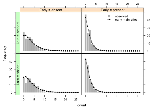
I improve the labeling on the factors defining the panels and add a legend.
xyplot(freq~count|factor(early, levels=levels(early), labels=paste('Early = ', levels(early), sep=''))+factor(late, levels=levels(late), labels=paste('Late = ', levels(late), sep='')), data=final.borer, type='h', lwd=8, col='grey', lineend=1, ylab='frequency', panel=function(x,y,subscripts){
panel.xyplot(x, y, type='h', lwd=8, col='grey',lineend=1)
panel.xyplot(x, final.borer$exp[subscripts], pch=16, cex=.7, type='o', col=1)},
key=list(x=.7, y=.85, corner=c(0,0), lines=list(col=c('grey',1), type=c('p','o'), pch=c(15,16), cex=c(1.2,.7), size=2), text=list(c('observed', 'early main effect'), cex=.9), divide=1)) -> my.graph
library(latticeExtra)
useOuterStrips(my.graph)
Parametric bootstrap
borer.p <- split(final.borer$p, final.borer$treatment)
myfunc <- function() {
out.obs <- as.vector(sapply(1:4, function(x) rmultinom(1, size=n[x], prob=borer.p[[x]])))
sum((out.obs-final.borer$exp)^2/final.borer$exp)
}
set.seed(50)
sim.data <- replicate(9999, myfunc())
actual <- sum((final.borer$freq-final.borer$exp)^2/final.borer$exp)
actual
[1] 74.0738
pearson <- c(sim.data, actual)
pval <- sum(pearson>=actual)/length(pearson)
pval
[1] 0.4984
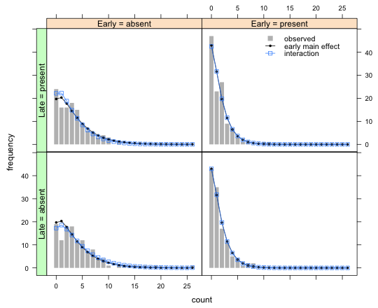
Question 3
The unconstrained model is the two-factor interaction model, or equivalently, a one-way model fit to the original treatment variable. We need to calculate the means, probabilities, and expected counts and add these to the graph of Question 2.
final.borer$mu2 <- predict(out.NB1, type='response', newdata=data.frame(early=final.borer$early, late=final.borer$late))
final.borer$p2 <- dnbinom(final.borer$count, mu=final.borer$mu2, size=out.NB1$theta)
final.borer$p2 <- final.borer$p2 + ifelse(final.borer$count==26, 1-pnbinom(26, mu=final.borer$mu2, size=out.NB1$theta), 0)
final.borer$exp2 <- final.borer$p2 * n[final.borer$treatment]
final.borer[1:8,]
count freq treatment early late mu p exp mu2 p2 exp2
Trt11 0 19 1 absent absent 3.6 0.16416474 19.699769 4.033333 0.14350498 17.220598
Trt12 1 12 1 absent absent 3.6 0.16930752 20.316902 4.033333 0.15471639 18.565967
Trt13 2 18 1 absent absent 3.6 0.14770788 17.724946 4.033333 0.14008190 16.809828
Trt14 3 18 1 absent absent 3.6 0.12104009 14.524810 4.033333 0.11876694 14.252032
Trt15 4 11 1 absent absent 3.6 0.09598139 11.517767 4.033333 0.09727647 11.673177
Trt16 5 12 1 absent absent 3.6 0.07458538 8.950245 4.033333 0.07799453 9.359343
Trt17 6 7 1 absent absent 3.6 0.05716880 6.860256 4.033333 0.06163656 7.396387
Trt18 7 8 1 absent absent 3.6 0.04338662 5.206394 4.033333 0.04820245 5.784294
xyplot(freq~count|factor(early,levels=levels(early), labels=paste('Early = ',levels(early),sep=''))+factor(late,levels=levels(late), labels=paste('Late = ', levels(late),sep='')), data=final.borer, type='h', lwd=8, col='grey', lineend=1, ylab='frequency', panel=function(x,y,subscripts){
panel.xyplot(x, y, type='h', lwd=8, col='grey', lineend=1)
panel.xyplot(x, final.borer$exp[subscripts], pch=16, cex=.6, type='o', col=1)
panel.xyplot(x, final.borer$exp2[subscripts], pch=22, cex=1, type='o', col='dodgerblue')
}, key=list(x=.7, y=.85, corner=c(0,0), lines=list(col=c('grey',1,'dodgerblue'), type=c('p','o','o'), pch=c(15,16,22), cex=c(1.2,.6, 1), size=2), text=list(c('observed','early main effect','interaction'), cex=.9), divide=1)
)->my.graph2
useOuterStrips(my.graph2)
Course Home Page