Assignment 11—Solution
Question 1
quinn <- read.csv('ecol 563/quinn1.csv')
quinn[1:4,]
Density Season Eggs
1 6 spring 1.167
2 6 spring 0.500
3 6 spring 1.667
4 6 summer 4.000
I create the variables needed for the BUGS program.
x1 <- as.numeric(quinn$Density==12)
x2 <- as.numeric(quinn$Density==24)
z <- as.numeric(quinn$Season=="summer")
y <- quinn$Eggs
n <- length(y)
The regression model we're fitting written in terms of dummy variables is the following.
where
 ,
,  ,
, 
The BUGS program that implements the two-factor interaction model is shown below.
model{
for(i in 1:n) {
y[i]~dnorm(y.hat[i],tau.y)
y.hat[i] <- b0 + b1*x1[i] + b2*x2[i] + b3*z[i] + b4*x1[i]*z[i] + b5*x2[i]*z[i]
}
b0~dnorm(0,.000001)
b1~dnorm(0,.000001)
b2~dnorm(0,.000001)
b3~dnorm(0,.000001)
b4~dnorm(0,.000001)
b5~dnorm(0,.000001)
tau.y <- pow(sigma.y,-2)
sigma.y~dunif(0,10000)
}
I create the objects needed by WinBUGS and run the model.
quinn.data <- list("n", "y", "x1", "x2", "z")
quinn.inits <- function() {list(b0=rnorm(1), b1=rnorm(1), b2=rnorm(1), b3=rnorm(1), b4=rnorm(1), b5=rnorm(1), sigma.y=runif(1))}
quinn.parms <- c("b0", "b1", "b2", "b3", "b4", "b5", "sigma.y")
setwd("C:/Users/jmweiss/Documents/ecol 563/models")
# WinBUGS
library(arm)
quinn.1 <- bugs(quinn.data, quinn.inits, quinn.parms, "quinnmodel.txt", bugs.directory = "C:/WinBUGS14", n.chains=3, n.iter=100, debug=T)
quinn.1 <- bugs(quinn.data, quinn.inits, quinn.parms, "quinnmodel.txt", bugs.directory = "C:/WinBUGS14", n.chains=3, n.iter=10000, debug=T)
# JAGS
library(R2jags)
quinn.1.jags <- jags(quinn.data, quinn.inits, quinn.parms, "quinnmodel.txt", n.chains=3, n.iter=10000)
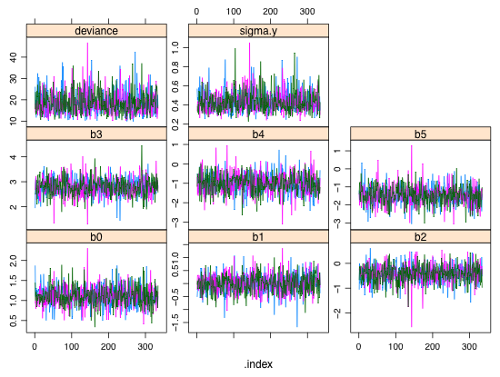
I display trace plots of the individual Markov chains for each parameter. The chains appear to be mixing wel and traversing the same region of parameter space.
xyplot(as.mcmc.list(quinn.1),layout=c(3,3))
|
| Fig. 1 Trace plots of individual Markov chains for each parameter. |
The summary table reveals that all the Rhat values are near 1 and the effective sample sizes (n.eff) are all large. All of this suggests that we are sampling from the posterior distributions of the various parameters.
round(quinn.1$summary,3)
mean sd 2.5% 25% 50% 75% 97.5% Rhat n.eff
b0 1.110 0.242 0.607 0.954 1.098 1.261 1.576 1.000 1000
b1 -0.001 0.352 -0.672 -0.228 0.004 0.231 0.689 1.000 1000
b2 -0.427 0.359 -1.161 -0.649 -0.415 -0.198 0.256 1.000 1000
b3 2.789 0.346 2.095 2.561 2.786 2.996 3.493 1.003 1000
b4 -1.008 0.502 -2.016 -1.311 -1.004 -0.697 -0.050 1.003 1000
b5 -1.470 0.506 -2.488 -1.788 -1.461 -1.180 -0.442 1.000 1000
sigma.y 0.432 0.107 0.280 0.357 0.413 0.484 0.682 1.000 1000
deviance 18.498 5.097 11.053 14.832 17.800 21.050 30.463 1.000 1000
Question 2
The 95% percentile credible intervals are returned in the summary table. The HPD intervals can be obtained by applying the HPDinterval function to the sims.matrix component of the bugs object. I collect them together in a single table.
colnames(quinn.1$sims.matrix)
[1] "b0" "b1" "b2" "b3" "b4" "b5" "sigma.y" "deviance"
out.hpd <- HPDinterval(as.mcmc(quinn.1$sims.matrix)[,1:7])
out.hpd
lower upper
b0 0.6335 1.602000
b1 -0.6425 0.704200
b2 -1.1030 0.305500
b3 2.1190 3.504000
b4 -1.9430 0.001201
b5 -2.5220 -0.488700
sigma.y 0.2626 0.650600
attr(,"Probability")
[1] 0.9500998
colnames(quinn.1$summary)
[1] "mean" "sd" "2.5%" "25%" "50%" "75%" "97.5%" "Rhat" "n.eff"
rownames(quinn.1$summary)
[1] "b0" "b1" "b2" "b3" "b4" "b5" "sigma.y" "deviance"
out.ci <- data.frame(quinn.1$summary[1:7, c("mean", "2.5%","97.5%")], out.hpd)
colnames(out.ci)[2:5] <- c('percent 2.5', 'percent 97.5', 'HPD 2.5', 'HPD 97.5')
round(out.ci,3)
mean percent 2.5 percent 97.5 HPD 2.5 HPD 97.5
b0 1.110 0.607 1.576 0.634 1.602
b1 -0.001 -0.672 0.689 -0.642 0.704
b2 -0.427 -1.161 0.256 -1.103 0.306
b3 2.789 2.095 3.493 2.119 3.504
b4 -1.008 -2.016 -0.050 -1.943 0.001
b5 -1.470 -2.488 -0.442 -2.522 -0.489
sigma.y 0.432 0.280 0.682 0.263 0.651
Question 3
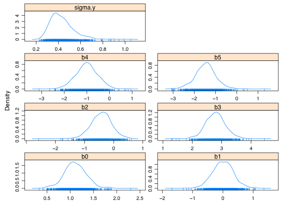
densityplot(as.mcmc(quinn.1$sims.matrix)[,1:7])
|
| Fig. 2 Estimated posterior densities for individual regression parameters |
Question 4
The individual means are obtained by assigning appropriate values to the dummy variables of the regression model. Table 1 below lists the dummy variable assignments and the corresponding expressions for the six means.
| Table 1 Individual means as determined by the regression model |
| Season |
Density |
x1 |
x2 |
z |
Mean |
| Spring |
6 |
0 |
0 |
0 |
 |
| Spring |
12 |
1 |
0 |
0 |
 |
| Spring |
24 |
0 |
1 |
0 |
 |
| Summer |
6 |
0 |
0 |
1 |
 |
| Summer |
12 |
1 |
0 |
1 |
 |
| Summer |
24 |
0 |
1 |
1 |
 |
Method 1
One way to obtain estimates of the means is to place expressions for the means in the BUGS program, add them to the parameter list, and rerun the model. The modified BUGS program is shown below.
model{
for(i in 1:n) {
y[i]~dnorm(y.hat[i],tau.y)
y.hat[i] <- b0 + b1*x12[i] + b2*x24[i]+b3*z[i] + b4*x12[i]*z[i] + b5*x24[i]*z[i]
}
b0~dnorm(0,.000001)
b1~dnorm(0,.000001)
b2~dnorm(0,.000001)
b3~dnorm(0,.000001)
b4~dnorm(0,.000001)
b5~dnorm(0,.000001)
tau.y <- pow(sigma.y,-2)
sigma.y~dunif(0,10000)
# means
mean1 <- b0
mean2 <- b0 + b1
mean3 <- b0 + b2
mean4 <- b0 + b3
mean5 <- b0 + b1 + b3 + b4
mean6 <- b0 + b2 + b3 + b5
}
I create a new parameters object adding the six means to the list of parameters to be returned. Rather than refit the model from scratch I use the last values of the different chains from the previous run as initial values for a new run.
quinn.parms2 <- c("mean1", "mean2", "mean3", "mean4", "mean5", "mean6", "b0", "b1", "b2", "b3", "b4", "b5", "sigma.y")
quinn.2 <- bugs(quinn.data, quinn.1$last.values, quinn.parms2, "quinnmodel.txt", bugs.directory = "C:/WinBUGS14", n.chains=3, n.iter=10000, debug=T)
round(quinn.2$summary,3)
mean sd 2.5% 25% 50% 75% 97.5% Rhat n.eff
mean1 1.102 0.249 0.586 0.948 1.112 1.252 1.577 1.000 1000
mean2 1.126 0.242 0.652 0.963 1.130 1.282 1.633 1.012 380
mean3 0.667 0.243 0.144 0.503 0.673 0.838 1.145 1.001 1000
mean4 3.884 0.262 3.367 3.713 3.869 4.057 4.394 1.000 1000
mean5 2.897 0.250 2.393 2.740 2.894 3.054 3.373 1.004 890
mean6 1.984 0.240 1.491 1.831 1.978 2.139 2.456 1.001 1000
b0 1.102 0.249 0.586 0.948 1.112 1.252 1.577 1.000 1000
b1 0.024 0.340 -0.623 -0.186 0.008 0.234 0.734 1.002 910
b2 -0.435 0.348 -1.128 -0.658 -0.424 -0.218 0.249 1.000 1000
b3 2.782 0.375 2.065 2.549 2.780 3.007 3.552 1.000 1000
b4 -1.011 0.516 -2.077 -1.304 -1.010 -0.705 -0.029 1.000 1000
b5 -1.465 0.518 -2.435 -1.793 -1.466 -1.130 -0.461 1.000 1000
sigma.y 0.422 0.098 0.284 0.351 0.407 0.473 0.650 1.004 460
deviance 18.147 4.925 10.900 14.580 17.325 21.007 29.107 1.002 810
Method 2
There's actia;;u no need to refit the model. We can obtain the posterior distributions of each parameter from the posterior distributions of b0, b1, b2, b3, b4, and b5. We just use the formulas for the means on the corresponding columns of the sims.matrix component of the bugs model that contains samples from the posterior distributions. Then we calculate the .025 and .975 quantiles using the values in each vector.
post.mean <- data.frame(mean1=quinn.1$sims.matrix[,"b0"], mean2=quinn.1$sims.matrix[,"b0"] + quinn.1$sims.matrix[,"b1"], mean3=quinn.1$sims.matrix[,"b0"] + quinn.1$sims.matrix[,"b2"], mean4=quinn.1$sims.matrix[,"b0"] + quinn.1$sims.matrix[,"b3"], mean5=quinn.1$sims.matrix[,"b0"] + quinn.1$sims.matrix[,"b1"] + quinn.1$sims.matrix[,"b3"] + quinn.1$sims.matrix[,"b4"], mean6=quinn.1$sims.matrix[,"b0"] + quinn.1$sims.matrix[,"b2"] + quinn.1$sims.matrix[,"b3"] + quinn.1$sims.matrix[,"b5"])
apply(post.mean, 2, mean)
mean1 mean2 mean3 mean4 mean5 mean6
1.109545 1.108993 0.682457 3.898386 2.889691 2.000862
apply(post.mean, 2, function(x) quantile(x,c(.025,.975)))
mean1 mean2 mean3 mean4 mean5 mean6
2.5% 0.6071675 0.620670 0.1728275 3.402343 2.402527 1.484685
97.5% 1.5759750 1.613133 1.1831560 4.424975 3.354662 2.562403
Comparing Bayesian and frequentist results
I fit the frequentist version of the model and obtain the 95% confidence intervals. I then append the Bayesian results.
out1 <- lm(Eggs~factor(Density)*Season, data=quinn)
out.g <- expand.grid(Density=levels(factor(quinn$Density)), Season=levels(quinn$Season))
freq <- data.frame(out.g,round(predict(out1, newdata=out.g, interval="confidence"),3))
bayes <- round(quinn.2$summary[1:6,c("mean", "2.5%", "97.5%")], 3)
both <- data.frame(freq, bayes)
names(both)[3:8] <- c('freq.mean', 'freq.low', 'freq.high', 'Bayes.mean', 'Bayes.low', 'Bayes.high')
both
Density Season freq.mean freq.low freq.high Bayes.mean Bayes.low Bayes.high
1 6 spring 1.111 0.635 1.587 1.102 0.586 1.577
2 12 spring 1.111 0.635 1.587 1.126 0.652 1.633
3 24 spring 0.695 0.219 1.171 0.667 0.144 1.145
4 6 summer 3.887 3.411 4.363 3.884 3.367 4.394
5 12 summer 2.887 2.411 3.363 2.897 2.393 3.373
6 24 summer 2.000 1.524 2.476 1.984 1.491 2.456
Course Home Page