Let y be the Poisson response, ![]() . Let x be a continuous predictor, z be a dichotomous variable coded 0 and 1, and w be the offset variable, then a generic Poisson regression model with an offset is the following.
. Let x be a continuous predictor, z be a dichotomous variable coded 0 and 1, and w be the offset variable, then a generic Poisson regression model with an offset is the following.
Exponentiating both sides and using the fact that exp(a + b + c) = exp(a + b) exp(c) we obtain the following.
Now z is a dummy variable coded 0 and 1. Thus we have two predicted rates depending on the value of z.
So with a dummy regressor in a Poisson regression with a log link, exponentiating the coefficient of the dummy regressor tells us the amount by which the mean rate is multiplied when we switch from the reference level (z = 0) to the other level (z = 1). Area, gear type, and time of day are dummy variables in the current model. So we just need to exponentiate their estimated coefficients to determine the multiplying factor. The regression coefficients and their exponentiated values are summarized in the table below.
The table summarizes the effect of area, gear type, and time of day on the estimated mean bycatch rate.
| Predictor | Reference level (z = 0) | Effect level (z = 1) | β | exp(β) | Interpretation |
| Area | North | South | 1.822 | 6.187 | The bycatch rate is 6.2 times greater in the South than the North. |
| Gear type | Bottom | Midwater | 1.918 | 6.805 | The bycatch rate is 6.8 times greater with midwater gear than with bottom gear. |
| Time of day | Day | Night | 2.177 | 8.816 | The bycatch rate is 8.8 times greater at night than during the day. |
The numbers reported by Manly are the same numbers shown at the bottom of the summary table of the model.
Null deviance: 335.096 on 42 degrees of freedomThe residual deviance is an appropriate goodness of fit statistic for a Poisson regression and has a chi-squared distribution only if the individual predicted counts are large. A seat-of-the-pants rule is that no more than 20% of the predicted counts should be less than 5 and none should be less than 1. I tabulate the predicted means obtained from the estimated model.
So 88.4% of the predicted counts are less than 5 and 76.7% of the mean counts are less than 1. Using the residual deviance as a goodness of fit statistic here is highly suspect.
The summary table of coefficient estimates is shown below.
Coefficients:The obvious problem is that the standard error for the season 1990-1991 effect estimate is 2439, over 100 times larger than the point estimate. Notice that all the other reported standard errors in the model are less 1, so this particular standard error is clearly anomalous. If we tabulate the bycatch by season we can see why this is happening.
In the 1990-1991 season there was no bycatch at all. This apparently is causing the software problems in estimating the variability of this effect. Given that we can't estimate the precision, we should probably not try to estimate the individual season effects.
To fit a random effects model we need to use the lme4 package and let the intercepts vary by season.
I modify the code we've used previously to display the predicted Poisson distributions for individual bycatch observations.
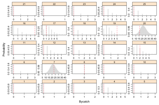 |
| Fig. 1(a) Predicted Poisson distributions with observed bycatch values superimposed. Observations 1–25. |
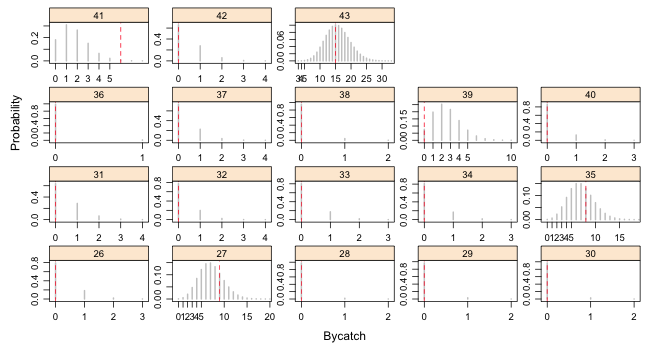 |
| Fig. 1(b) Predicted Poisson distributions with observed bycatch values superimposed. Observations 26–43. |
From the graphs we can see that observations 16, 19, and 41 are poorly described by the model. We can test this formally by calculating upper and lower-tailed p-values. I carry out a two-tailed test and compare each p-value against α = 0.025
There are three significant results. Because 3 out of 43 = 6.9%, this is a little bit larger than we'd expect by chance. Fig. 2 displays the upper and lower-tailed p-values separately. (Note: it's not possible here to display them in a common plot because for most of the observations both the lower- and upper-tailed p-values are large, greater than 0.9.)
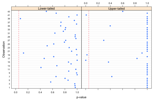 |
| Fig. 2 Upper- and lower-tailed p-values for individual observations with respect to their predicted Poisson distributions. |
I first identify the observations with significant p-values.
I extract the residuals, label them, and display them in decreasing order.
So the significant p-values correspond to the observations with the largest Pearson residuals. Thus the residuals can serve as goodness of fit statistics in the sense that we're using it here.
I refit the random intercepts model but this time treating log(Tows) as a covariate rather than an offset.
There are three ways to determine whether a model with log(Tows) as a covariate is superior to a model in which log(Tows) is treated as an offset: likelihood ratio test, Wald test, and AIC.
The Poisson random intercepts model with log(Tows) as an offset is nested in the Poisson random intercepts model with log(Tows) treated as a covariate. In the offset model we're setting the coefficient equal to 1. Thus we can formally compare the models using a likelihood ratio test. The hypothesis test this yields is the following.
H0: β = 1
H1: β ≠ 1
We can carry out the test with the anova function (or by hand by using twice the difference in the loglikelihoods).
So the likelihood ratio test is not significant. Thus 1 is a legitimate value for the coefficient suggesting that treating log(Tows) as an offset is reasonable.
A second test we can carry out is a Wald test. The Wald test shown in the summary table is not useful here because it tests H0: β = 0, whereas we want to test whether H0: β = 1. Testing that a parameter has a specific value is equivalent to determining whether that value lies in a confidence interval for that parameter. We can construct the confidence interval by hand using the output from the summary table. The confidence interval takes the form ![]() .
.
Because 1 does not lie in the 95% confidence interval a Wald test rejects the null hypothesis that the coefficient of log(Tows) is equal to one. Therefore according to the Wald test log(Tows) should not be treated as an offset. Alternatively to carry out the test formally we need to calculate the following test statistic.
The two-tailed p-value is calculated as follows.
I compare the models using AIC.
Although the AIC values are close, the model in which the coefficient of log(Tows) is estimated has a lower AIC than a model in which log(Tows) is treated as an offset, even though we have to estimate one more parameter. Thus our results are ambiguous. Both the Wald test and AIC favor treating log(Tows) as a covariate while the likelihood ratio test favors treating log(Tows as an offset. This is not surprising given the arbitrariness of the α = .05 cut-off.
I calculate the upper and lower-tailed p-values for the new model.
So, the number of significant p-values has been reduced from three to two. I examine the largest residuals from this model.
So the three largest positive residuals are all reduced from what they were in the offset model.
| Jack Weiss Phone: (919) 962-5930 E-Mail: jack_weiss@unc.edu Address: Curriculum for Ecology and the Environment, Box 3275, University of North Carolina, Chapel Hill, 27599 Copyright © 2012 Last Revised--November 25, 2012 URL: https://sakai.unc.edu/access/content/group/3d1eb92e-7848-4f55-90c3-7c72a54e7e43/public/docs/solutions/assign10.htm |