Assignment 1— Solution

Question 1

I read in the data, convert Density to a factor, and fit a two-factor analysis of variance model with Eggs as the response and Season, Density, and their interaction as predictors.

Response: Eggs
               Df  Sum Sq Mean Sq F value    Pr(>F)   
Density         2  4.0019  2.0010  13.984 0.0007325 ***
Season          1 17.1483 17.1483 119.845 1.336e-07 ***
Density:Season  2  1.6907  0.8454   5.908 0.0163632 * 
Residuals      12  1.7170  0.1431                     
---
Signif. codes:  0 ‘***’ 0.001 ‘**’ 0.01 ‘*’ 0.05 ‘.’ 0.1 ‘ ’ 1

Based on the output we see that there is a significant interaction between Density and Season. This means that the effect of Density on egg count varies with Season (and vice versa). We can examine the summary table to try to understand the nature of this interaction.

Residuals:
     Min       1Q   Median       3Q      Max
-0.61133 -0.16167 -0.04217  0.09892  0.55567

Coefficients:
                         Estimate Std. Error t value Pr(>|t|)   
(Intercept)             1.1113333  0.2183934   5.089 0.000267 ***
Density12              -0.0003333  0.3088549  -0.001 0.999157   
Density24              -0.4166667  0.3088549  -1.349 0.202221   
Seasonsummer            2.7753333  0.3088549   8.986 1.12e-06 ***
Density12:Seasonsummer -0.9996667  0.4367868  -2.289 0.041029 * 
Density24:Seasonsummer -1.4700000  0.4367868  -3.365 0.005617 **
---
Signif. codes:  0 ‘***’ 0.001 ‘**’ 0.01 ‘*’ 0.05 ‘.’ 0.1 ‘ ’ 1

Residual standard error: 0.3783 on 12 degrees of freedom
Multiple R-squared: 0.9301,            Adjusted R-squared: 0.9009
F-statistic: 31.93 on 5 and 12 DF,  p-value: 1.561e-06

From the output it appears that there is no Density effect in spring (the Density12 and Density24 coefficients are not significantly different from zero) but there is a Density effect in summer (the two interaction terms are significant). We'll explore this issue further in Question 3.

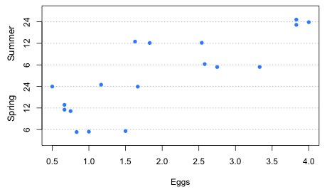
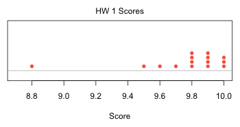
Some people examined the issue of variance homogeneity. For that we need to create a variable that identifies the individual treatments. This can be accomplished with the paste function that concatenates the character values of two variables. I then plot the Egg counts against the new treatment variable in a dot plot.

Fig. 1  Dot plot of the response variable separately by treatment

While there are some differences in variability across treatment we only have three observations per treatment, not enough to obtain a reliable estimate of variability. We can test for variance heterogeneity but we won't have much power. Given how unreliable our variance estimates are I just report the results from the robust tests, Fligner's and Levene's tests, below. Neither test statistic is close to being statistically significant.

data:  quinn$Eggs by quinn$trt
Fligner-Killeen:med chi-squared = 4.1871, df = 5, p-value = 0.5228

Question 2

To display the two-factor interaction we have a choice. We can plot Density on the x-axis and show separate profiles for each Season, or we can plot Season on the x-axis and shows separate profiles for each Density. Generally it's useful to do both, but because Density is an ordinal variable it makes more sense to plot Density on the x-axis so we take advantage of the natural order of the three Density categories.

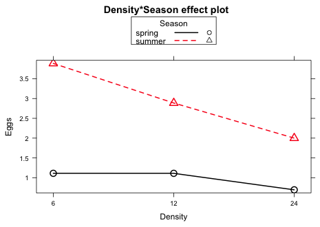
Fig. 2  Plot of the significant two-factor interaction between Season and Density

The interaction apparently derives from the fact that there is a much stronger negative effect of Density on egg count in the summer than there is in the spring.

Question 3

Because Density has three levels it was entered into the analysis of variance model as two dummy variables. Season with two levels was entered as a single variable. The default definitions used by R are the following.

, , 

The regression model corresponding to the two-factor interaction model is the following.

The coefficient summary table for the model generated by R is shown below.

Using the regression equation and the estimates reported in the summary table we can draw the following conclusions.

1. When the Density = 6 and Season = 'Spring', x₁ = x₂ = z = 0. So, our regression model is μ = β₀. Thus the intercept, 1.11, corresponds to the mean egg count in Spring when the Density is 6.
2. When Season = 'Spring', z = 0, and the regression equation is the following: . This yields the following estimates of the mean egg count at the three different densities

Season	Density	x1	x2
Spring	6	0	0
Spring	12	1	0
Spring	24	0	1

From the summary table β₁ = –0.0003 and β₂ = –0.4167. Both of these effects are negative so mean egg count decreases as Density increases. On the other hand the summary table reports that neither of these effects are statistically significant. Thus the mean egg count in Spring when density is 12 is not significantly different from what it was when Density is 6. Similarly the mean egg count when density is 24 is not significantly different from what it was when Density = 6.

3. When Density = 6 and Season = 'Spring', x₁ = x₂ = 0 and z = 1. Thus the regression model is . We have the following estimates of the mean egg count in Spring and Summer when Density = 6.

Season	Density	z
Spring	6	0
Summer	6	1

The parameter β₃ represents the difference in mean egg counts, Summer – Spring. From the summary table we see that β₃ = 2.7753 and it is significantly different from zero. Thus we conclude that the mean egg count is significantly higher in Summer than in Spring when Density = 6.

4. The interaction terms are a bit more involved to explain. Table 3 compares the coefficients from an additive model (a model without the interaction terms) with those from the interaction model when Season = 'Summer'.

Season	Density	x1	x2	z	Additive model	Interaction model
Summer	6	0	0	1
Summer	12	1	0	1
Summer	24	0	1	1

Fig. 3 graphically contrasts the predictions of the additive model (one with only the main effects of Season and Density) to the interaction model. Because the reported estimates of the parameters β₄ and β₅ are negative, the interaction model summer profile lies below the additive model summer profile.

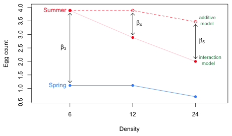
Fig. 3  Contrasting the additive and interaction models for Season and Density

In the additive model the mean profiles for Spring and Summer are parallel. The regression coefficients β₄ and β₅ in the interaction model are the deviations from additivity (and hence parallelism). The fact that these effects are estimated to be negative (–1.00 and –1.47) and statistically significant indicates that the Season effect is significantly reduced when Density is 12 or 24 than what it is when Density is 6. When density = 6 there is a very large season effect of β₃ = 2.775. When density = 12 the season effect is not as large (2.7753 – 0.9997 = 1.776). When density = 24 the season effect is even smaller (2.7753 – 1.47 = 1.31). These effects of density on the season effect are statistically significant.

So we have two interpretations of the interaction. One interpretation is that Density has a marked negative effect on mean egg count in the Summer, but not in Spring. The other interpretation is that the increase in egg count from spring to summer that we see when density is 6 gets significantly reduced when density = 12 and even more so when density = 24.

Question 4

I obtain 1000 simulations from the two-factor interaction model.

Following the hint I take the minimum of the simulations.

The simulations returned a negative value. Given that the response variable is egg count, a positive whole number, a negative value is an unreasonable prediction. The simulations produced by the simulate function are organized as columns. I count up the number of simulations that produced one or more negative values. I use the apply function to sum up the number of negative values in each column. I then tabulate the results.

So 107 simulations yielded a single negative value (out of 18) while three yielded two negative values. Thus 11% of the simulations returned one or more silly values. We can count up the number of negative values and divide by the total number of simulated observations to obtain the overall percentage of silly values.

So, about 0.6% of the simulated values are negative, not a large number, but still indicating that perhaps the model is formulated incorrectly. We'll investigate this further later in the course after we have added more statistical tools to our arsenal.

R code used to produce Fig. 3

Course Home Page