
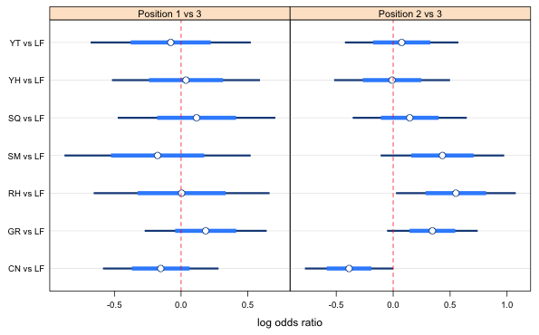
Fig. 1 Preliminary graph of the log odds ratios using the minimum confidence level for the pairwise comparisons confidence intervals.
There are many ways to do this. They all involve two operations that we then combine into a single step. Here are a few possibilities.
We have a categorical response with three categories. I fit a multinomial model with treatment as the predictor. I then compare it to a model containing only an intercept using a likelihood ratio test.
Response: position
Model Resid. df Resid. Dev Test Df LR stat. Pr(Chi)
1 1 454 5519.935
2 treatment 440 5461.129 1 vs 2 14 58.80575 1.898106e-07
The test is highly significant. There is evidence of a treatment effect.
A goodness of fit test can be obtained by comparing the current model to a saturated model, a model that estimates separate parameters for each multinomial observation. The variable trial in the data set identifies the 76 different multinomial observations in this experiment. I enter it as the sole predictor in a multinomial model.
Response: position
Model Resid. df Resid. Dev Test Df LR stat. Pr(Chi)
1 treatment 440 5461.129
2 trial 304 5134.452 1 vs 2 136 326.6776 0
So it appears that we have a significant lack of fit. This test does have some minimal cell size restrictions that must be met in order for the chi-square distribution of the test statistic to be valid. The general rule is that the number of expected counts less than 5 should not exceed 20%. I obtain the totals for each trial and the predicted probabilities on each trial and then use these to obtain the expected counts.
So only about 2% of the expected counts are less than 5. The goodness of fit test is valid.
Different fish were used on different days and there may have been changes in protocol from day to day. Thus it makes sense to treat day as a blocking variable and include day as a factor in the model. The experiment was carried out over 14 days with not every treatment tested on each day. So, it's not possible to include an interaction between treatment and day with these data. Day has numeric values so I have to explicitly declare it as a factor when fitting the model.
Response: position
Model Resid. df Resid. Dev Test Df LR stat. Pr(Chi)
1 treatment + factor(day) 414 5322.629
2 trial 304 5134.452 1 vs 2 110 188.1774 5.046884e-06
The fit has improved but there is still a significant lack of fit.
Two assumptions of a multinomial experiment are the following.
Independence is clearly violated. We are told that this is a repeated measures design. The same fish were observed 12 times and their positions at these times were recorded. Given this it's pretty clear the observations for a given trial are not independent because we are repeatedly using observations from the same fish as well as different fish. Furthermore the three fish used on each trial can observe and respond to each other. This also violates independence.
It's also possible that the position selection probabilities of individual fish are not constant because if habituation occurs. If the fish grow accustomed to the presence of the predator fish during a trial their behavior may change. We're also told the same fish were reused during the course of the day, so it's possible that the fish had different selection probabilities early in the day than late in the day.
To fit a multinomial model as a Poisson model we need to include specific variables that enforce the multinomial constraints. Here's a portion of the what the raw data look like when organized as multinomial trials.
To obtain a multinomial model we need to include the variable trial as a predictor (to fix the row sums) and the variable position as a predictor (to fix the column sums). The null multinomial model when fit as a Poisson model is the following.
This is called the independence model. It claims that trial and position are unrelated. So this is our "nothing's going on" model equivalent to the intercept-only multinomial model above. If we look at the predicted counts (fitted values) from this model we'd see that each trial is predicted to have the same fraction of 1s, 2s, and 3s.
The two additive terms in the model just define the constraints of the experimental design so that our predictions have the same row and column totals as the data have. When you fit the multinomial model with the multinom function these constraints are already built in so you just need to include an intercept as the only predictor.
The independence model is uninteresting. If we add trial:factor(position) to the independence model we let every trial have its own values for position (still subject to the constraints of the experiment). The fractions of 1s, 2s and 3s are now different in every trial. This is also an uninteresting model. It says everything is different from everything else. It is the saturated model. It estimates one parameter for each cell of the table, a total of 228 parameters, and fits the data perfectly.
Our goal is to replace trial:factor(position) with something more interesting and still have a model that fits the data. Rather than letting each trial have its own unique fractions for each position, we could force those trials experiencing the same treatment to have the same fractions but different from the fractions in trials receiving different treatments. To fit this model we replace the term trial:factor(position) with treatment:factor(position).
To include the blocking variable day in the model I add the interaction term factor(day):factor(position) to the model.
We can verify these models are correct by carrying out the goodness of fit test we did previously and observe that we get the same likelihood ratio statistic here as we did using the multinom function.
Model 1: freq ~ factor(position) + trial + treatment:factor(position) +
factor(day):factor(position)
Model 2: freq ~ factor(position) + trial + trial * factor(position)
Resid. Df Resid. Dev Df Deviance Pr(>Chi)
1 110 188.18
2 0 0.00 110 188.18 5.047e-06 ***
---
Signif. codes: 0 ‘***’ 0.001 ‘**’ 0.01 ‘*’ 0.05 ‘.’ 0.1 ‘ ’ 1
Finally then, to fit the desired quasi-Poisson model I change the family argument of this last model to quasipoisson.
To generate the estimates with the correct reference group for treatment we need to redefine treatment as a factor specifying "LF" as the reference group. As was explained in the hints it is unnecessary to to do this for position. The default order of position will surprisingly give us what we want.
I refit the model using the new treatment variable.
We need the estimates that involve the interaction with treatment. I use the grep function to locate those rows in the coefficient table that contain the string 'treat'.
I extract just this portion of the coefficient summary table and the corresponding variance-covariance matrix.
The panel graph we want displays the two position comparisons in separate panels so it will be convenient to have things sorted so the position 1 estimates are together followed by the position 2 estimates.
I begin to assemble the data frame we need for plotting purposes.
I add the 95% confidence intervals.
Technically we should use a t-distribution with degrees of freedom taken from the model, but the difference here is slight.
Next we need to compute the confidence levels for the pairwise comparisons. I collect the functions we've previously written for this purpose.
We need to use this function one panel at a time specifying the corresponding rows from the coefficient matrix, first 1:7 and then 8:14. Each run involves pairwise comparisons between 7 estimates.
The confidence levels range from 0.67 to 0.79 so we're going to need to do some experimenting in setting the levels. I start by using the lowest confidence level in each panel.
We're ready to produce the panel graph. First I collect the names of the predator fish in the order they're being presented in the coefficients table, omitting the lionfish LF.
Next I produce the graph using the current choices for the pairwise confidence levels.
|
|---|
Fig. 1 Preliminary graph of the log odds ratios using the minimum confidence level for the pairwise comparisons confidence intervals. |
Everything overlaps in the first panel so we have nothing more to do there. If we increase the confidence levels the overlap will just increase. In the second panel we see that the first log odds ratio looks different from the next four. The confidence level we're using, 0.67, is only correct for the first comparison. The comparison that looks closest to being not significant is 1 vs 5. According to the vals1 vector the confidence level for this comparison should be 0.73, so I try that next.
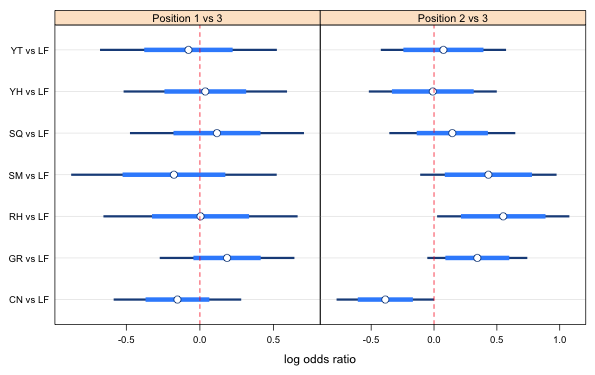
The graph using this confidence level is shown below.
 |
|---|
Fig. 2 Point estimates, 95% confidence intervals (thin bar), and variable level confidence intervals suitable for making all pairwise comparisons of displayed estimates. A 67% confidence level is used for the position 1 vs 3 comparison and a 73% confidence level is used for the position 2 versus 3 comparison. |
With that choice nothing else looks different that would require raising the confidence level except perhaps a comparison of the RH vs LF and the YH vs LF intervals. If we look at the table of confidence levels (below I've labeled then by what comparison they correspond) we see that the confidence level for the comparison of 3 versus 6 is 0.79 and is in position 14 of the vector.
If we change all the levels to 0.79 then the CN vs LF and SQ vs LF comparison is no longer significant. I instead change only the levels for the two observations involved in the comparison, RH and YH.
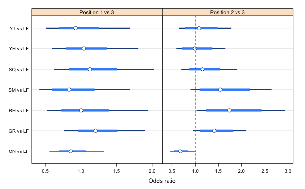
The final graph is shown below.
 |
|---|
Fig. 3 Point estimates, 95% confidence intervals (thin bar), and variable level confidence intervals (thick bars) that are suitable for making all pairwise comparisons of displayed estimates. A 67% confidence level is used for all the position 1 vs 3 comparisons and a 73% confidence level is used for the position 2 versus 3 comparisons. The only exceptions are for RH vs LF and YH vs LF intervals for which 79% confidence levels are shown. |
I exponentiate the point estimate and the confidence intervals and generate the new graph.
 |
|---|
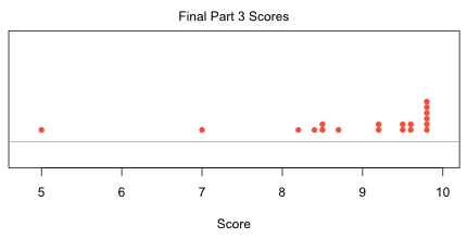
Fig. 4 Odds ratios estimates for different predators versus lionfish separately for position 1 versus position 3 and position 2 versus position 3. |
None of the odds ratios for the position 1 versus position 3 comparison are significant. All of the 95% confidence intervals include an odds ratio of 1. Thus the ratio of times prey turn toward a predator or turn away from a predator are the same for any predator when compared to lionfish, even for the control in which no predator was present at all. The only significant odds ratios were found for the position 2 versus position 3 comparisons. If position 2 indicates that the prey are taking greater notice of the predator, then lionfish are significantly (in truth the p-value just exceeds 0.05) scarier than a control (a cage with nothing in it) while the red hind is significantly scarier than a lionfish. No other odds ratios were statistically significant.
It's worth noting that if we had used a Poisson rather than a quasi-Poisson distribution here, we would have found the odds ratios of LF with CN, GR, RH, and SM to all be statistically significant for position 2 versus position 3. The quasi-Poisson gives us more conservative results, which is probably justified here given that we know the model has a significant lack of fit.
Apparently the assumption that the fish would turn toward the predator when frightened is incorrect. The ratio of times a fish is in position 1 versus position 3 is not affected by the predator's identity (at least when using lionfish as the reference group). This is true even when there is no predator present at all. What we see instead is that a frightened fish turns perpendicular to the predator (position 2). This makes sense if the eyes of this fish are laterally placed so that the fish lacks good binocular vision. What supports this is that the only time the empty cage (control) versus lionfish comparison yielded an .odds ratio that was less than 1 was for the position 2 versus position 3 comparison (and not for the position 1 versus position 3 comparison).
The pairwise comparisons are not particularly interesting here. We see from the pairwise comparisons that individually the odds ratios for the different predators cannot be distinguished from each other. Still, four of them are significantly greater than the lionfish vs control odds ratio (red hind, grouper, schoolmaster, and squirrelfish) but two were not (yellowtail and yellowhead). So even though only the red hind was significantly scarier than the lionfish, there is a weak suggestion that the predators perhaps fall into two groups: lionfish, yellowhead, yellowtail in one group and grouper, red hind, schoolmaster, and squirrelfish in a second group.
Of the fish used in this experiment the red hind is the most imposing and was expected to be the scariest predator. It is interesting that although none of the other predator ORs are significant, their point estimates do exceed 1. The only exception to this is the yellowhead (OR = 0.99) which mostly eats invertebrates anyway. The rankings are close to what the researchers would have guessed based on their knowledge of these fish. The results suggest that while lionfish are not ignored by their potential prey they do currently rank at the low end of their concerns. The lack of significance of most of the ORs probably results from the inefficient experimental design (evidence for which is found in the persistent lack of fit). Fortunately the researchers measured other behavioral attributes that confirmed the weak trends that are shown here.
| Jack Weiss Phone: (919) 962-5930 E-Mail: jack_weiss@unc.edu Address: Curriculum for the Environment and Ecology, Box 3275, University of North Carolina, Chapel Hill, 27599 Copyright © 2012 Last Revised--May 4, 2012 URL: https://sakai.unc.edu/access/content/group/2842013b-58f5-4453-aa8d-3e01bacbfc3d/public/Ecol562_Spring2012/docs/solutions/finalpart3.htm |