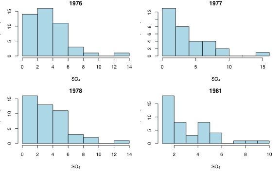
Fig. 1 Histograms of SO4 concentration in each year
Read in the data.
The data are currently in "lake-level" format in which each lake has a single record. We need to put this into "lake-period" format with multiple records for each lake, in this case one record for each measurement occasion. This requires unlisting the records X1976, X1977, X1978, and X1981 stacking them into a single column, replicating the Lake, Latitude, and Longitude variables four times, and adding a new column that lists the year the measurement was taken.
There are a number of guidelines for helping us choose a probability model for the response variable SO4. I repeat some of these here.
Clearly SO4 is a continuous variable and, being a concentration, is bounded below by zero (but in principle unbounded above). Three continuous distributions mentioned at various times in the course are the normal, lognormal, and gamma distributions. Both the lognormal and gamma are positive data distributions and are bounded below by zero, while the normal distribution is unbounded. Of course if the data are displaced far enough from zero, then the fact that the normal distribution is unbounded below may not be a problem. The easiest way to obtain a lognormal distribution is to log-transform a response variable and assume the log-transformed variable has a normal distribution.
Because the goal is to model SO4 concentration against year the probability model we're seeking must hold at each year separately rather than in the aggregate. Because both the lognormal and gamma distributions tend to be skewed while the normal is symmetric, a histogram of SO4 concentration at each year is a useful display.
Fig. 1 Histograms of SO4 concentration in each year
From Fig. 1 it's pretty clear that a normal distribution is likely to be inappropriate. The actual distributions are skewed and have many values close to zero. Thus a model based on a normal distribution is likely to predict negative concentrations. Both the lognormal and gamma distributions have the same mean-variance relation (quadratic), so the best way to evaluate them is to actually use them in a model and compare the results with AIC. Even though we know a normal model is probably inappropriate I include it among the candidate models.
I start by fitting each model with year as a linear predictor. The normal and lognormal models can be fit with lm, the lognormal by first log-transforming the response SO4. The gamma distribution is fit with glm and the family=Gamma argument.
The log-likelihood of the log-transformed model is not directly comparable to models with an untransformed response without additional work. We wrote a function in lecture 11 called norm.loglike5 that carries out the necessary steps and I reproduce it below. We did two versions of the function. Here we need the version that is based on a probability density function (rather than a probability) because we've comparing density functions.
To get this function to work we need to give it a version of the data set in which the missing values of the response are removed. (These observations are automatically removed by the lm function when a model involving them is fit.) We can do this by subsetting the data set using the !is.na( ) construction. The first argument to the norm.loglike5 function is the model, the second is 0 because we didn't add a constant to the response, and the third is the response variable with missing observations removed.
Each of the models has three estimated parameters: (β0, β1, and σ2) for the normal and lognormal and (β0, β1, and scale) for the gamma, so we could just as well compare log-likelihoods rather than AIC.
The lognormal model has the lowest AIC by a sizeable amount, so we'll proceed with a lognormal probability model for the response. Fig. 2 shows the three fitted distributions separately by year superimposed on histograms of the data.
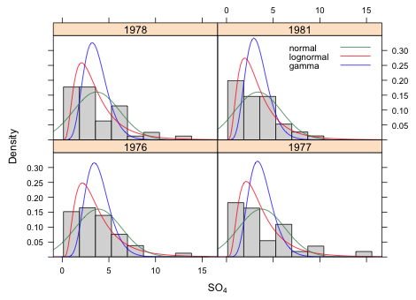 |
Fig. 2 Different probability distributions fit to sulfate concentration separately by year using a linear year model |
The variable year has four unique values. Hence there are a limited number of choices for the linear predictor. Without any theory to guide us we can
Each model was fit assuming a lognormally distributed response. AIC can be used to compare the models without any adjustment because all three models use the same response, log SO4.
Clearly the linear model is to be preferred. It has both the lowest AIC and is simpler. To see what's going on I graph the data (jittered) and superimpose the three models. For the separate means model I just plot the estimated mean at each year as predicted by the model. The graphs of the three models are indistinguishable.
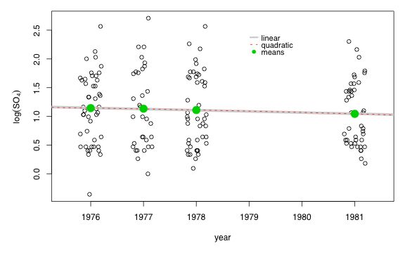
Fig. 3 Three lognormal models using different versions of the linear predictor for year
Our conclusions remaining the same even if we use a normal or a gamma probability model for the response. A model linear in year is best.
For comparison I obtain the AIC of the lognormal models on the scale of the response variable.
Table 1 summarizes the common pooling models that were fit.
Model |
Linear predictor | k |
log-likelihood |
AIC |
lognormal |
linear year | 3 |
–342.018 |
690.035 |
| quadratic year | 4 |
–342.015 |
692.030 |
|
| categorical year | 5 |
–342.014 |
694.028 |
|
gamma |
linear year | 3 |
–349.840 |
705.681 |
| quadratic year | 4 |
–349.708 |
707.416 |
|
| categorical year | 5 |
–349.605 |
709.210 |
|
normal |
linear year | 3 |
–390.424 |
786.849 |
| quadratic year | 4 |
–390.333 |
788.667 |
|
| categorical year | 5 |
–390.239 |
790.478 |
Of course it is possible that some weird transformation of year is preferable to what we've done. To assess that possibility I plot the residuals from the linear model against year and superimpose a lowess curve.

Fig. 4 Plot of residuals from model linear in year against the predictor "year"
The plot provides no evidence that form of the linear predictor is inadequate. It's worth noting at this point that the modeled relationship between log(SO4) and year is not statistically significant.
Call:
lm(formula = l4og(SO4) ~ year, data = newlakes)
Residuals:
Min 1Q Median 3Q Max
-1.50496 -0.52462 -0.08062 0.52028 1.58027
Coefficients:
Estimate Std. Error t value Pr(>|t|)
(Intercept) 41.66739 49.32240 0.845 0.399
year -0.02051 0.02493 -0.822 0.412
Residual standard error: 0.6167 on 166 degrees of freedom
Multiple R-Squared: 0.004057, Adjusted R-squared: -0.001942
F-statistic: 0.6763 on 1 and 166 DF, p-value: 0.4120
The basic structure possessed by these these data is that they consist of repeated measures on individual lakes. Due to local geology and edaphic factors, we should expect measurements coming from the same lake, even separated by a time interval of a year or more, to be more similar to each other than to observations coming from other lakes. This provides the potential for what we've called observational heterogeneity—differing degrees of variability in subsets of observations. Observe that the repeated measures aspect of these data was imposed at the design level. Structure that arises from the sampling design must be accounted for in the analysis.
In addition to temporal correlation there is the possibility of spatial structure in these data as a function of their geographic proximities. We might expect lakes that are close to each other to share a similar chemistry. I consider structure of this sort to be inadvertent structure in these data. It arises because lakes are fixed objects that occupy space and the problem of their varying proximities will be an issue in even the most well-designed random selection scheme. The spatial structure may turn out to be important, but it is not intrinsic to the experimental design. As a result we'll account for the designed structure first and then deal with the spatial structuring if necessary.
The ideal way to display the temporal structure of these data is in a lattice graph in which we plot the SO4 concentration versus year separately for each lake. Because we've already seen that a log transformation of the SO4 concentration is justified, the most useful lattice graph plots log(SO4) versus year.
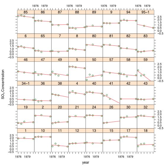
Fig. 5 Lattice graph displaying the repeated measures structure of the data set
As Fig. 5 indicates there is a dramatic difference in baseline SO4 concentrations across lakes. This is reflected in the widely different values of the intercepts in the different regression lines. We also see some evidence for heterogeneity in slopes across the lakes. The natural way to handle structured data such as these is with a multilevel model. Fig. 5 coupled with our early work using the complete pooling model suggests that a linear model relating log(SO4) concentration to continuous time should be an adequate starting point.
The correct place to begin when fitting a multilevel model is with the common pooling (unconditional means) model. The common pooling model includes only an intercept but does allow that intercept to vary among the different lakes. It serves to partition the variance between and among lakes and acts as a benchmark that allows us to assess where most of the variability lies—between lakes or between years for the same lake. The common pooling model is formulated as follows.
where ![]()
Written as a composite equation it takes the following form.
It's the latter form that matches the syntax used by R's lme function.
The unconditional means model is of interest only for its variance components. From these we can calculate the intraclass correlation coefficient.
I calculate this for the lakes data using output from VarCorr.
So we see that 91% of the variability in log(SO4) concentrations occurs between lakes rather than within lakes across years. Put another way measurements from the same lake exhibit a correlation of 0.91. This is dramatic evidence that a multilevel model is needed here and argues strongly against using a common pooling model.
The next step is to add the predictor year. As we've seen the individual trend lines in Fig. 4 exhibit quite a bit of variability in their intercepts. Thus a natural second model to consider is a random intercepts model, a linear population model in which the intercepts of the regression lines for individual lakes are allowed to vary but they still share a common slope.
where ![]()
Written in composite form random intercepts model is the following.
Written this way it matches the syntax used by R's lme function.
Observe the dramatic decrease in AIC relative to the common pooling model, strong evidence that we need to account for the repeated measures structure of the data set. (The AIC values are directly comparable here because all models use log(SO4) as the response.) The random intercepts model exhibits a more modest decrease in AIC relative to the unconditional means model indicating that the inclusion of year has improved the fit of the model somewhat. Next we examine the variance components.
As measured by the small relative reduction in level-1 variance, year accounts for only a modest amount of within-lake variability.
So we've explained only 8% of the within-lake variability by including year as a predictor. Still the predictor year is statistically significant.
Random effects:
Formula: ~1 | lake
(Intercept) Residual
StdDev: 0.5774515 0.1689954
Fixed effects: log(SO4) ~ year
Value Std.Error DF t-value p-value
(Intercept) 45.76822 13.897196 119 3.293342 0.0013
year -0.02259 0.007026 119 -3.215169 0.0017
Correlation:
(Intr)
year -1
Standardized Within-Group Residuals:
Min Q1 Med Q3 Max
-4.02214991 -0.47329909 -0.05670254 0.55159957 3.33206296
Number of Observations: 168
Number of Groups: 48
Another model we might consider is a random slopes and intercepts model. The lattice graph of Fig. 5 suggests there is some variability in individual slopes. Unfortunately this model is very difficult to fit. One of the pernicious features of fitting mixed effects models is that it's not always clear that there things have gone wrong. Recall that the random slopes and intercepts model takes the following form.
where  .
.
In composite form the equations reduce to the following.
The following function call fits the random slopes and intercepts model in R.
If we look at the variance components of this model we see the following.
Based on the displayed correlation of 0 between the random slopes and intercepts and the estimated variance component of the slopes that is approximately 0 we see that R has converged to a solution in which the slopes don't vary. If we compare the log-likelihoods of the random slopes and intercepts model with that of the random intercepts model we see that they are identical!
It is extremely unlikely that introducing two additional parameters to the model has had no effect on the log-likelihood. Given that we've already seen from our lattice plot that the slopes do vary between lakes we should surmise that lme has converged to a local solution (the solution of the random intercepts model) rather than a global solution.
To remedy the situation we can try reparameterizing the predictor, perhaps by centering, and if that doesn't work to modify some of the control settings of the maximization algorithm. In the next model run I shift the origin to 1976, increase the default iteration settings, and switch the optimization method to optim.
This time the log-likelihood has increases. However this model does not beat the random intercepts model.
Another model we might consider is a random slopes model although the lattice graph of Fig. 5 suggests there isn't much variability in the slopes. A random slopes model is one in which the slopes of the regression lines for individual lakes are allowed to vary but they still share a common intercept.
where ![]()
Written in composite form the random slopes model is the following.
To fit this model we need to explicitly remove the intercept from the random argument of lme.
The table below summarizes the results. Because all the models being compared have log(SO4) as the response we can use AIC applied directly to the model object to compare them. The AIC values reported here cannot be used to compare these models against models with other probability models for the response. Note: the norm.loglike5 function we used above does not return the correct AIC when random effects are involved. A different function is necessary.
Lognormal Model |
Predictor |
# parameters |
log-likelihood (for log y) |
AIC |
| common pooling | year |
3 |
–159.159 |
318.318 |
| unconditional means | — |
3 |
–33.882 |
73.763 |
| random intercepts | year |
4 |
–28.866 |
65.732 |
| random slopes and intercepts | year |
6 |
–27.192 |
66.383 |
| random slopes | year |
4 |
–28.945 |
65.890 |
A model I don't include in the above list is the separate intercepts model, a model that estimates a separate intercept for each lake. This model would be fit as follows.
In this model we would end up estimating 45 additional parameters, one intercept for each lake. Not surprisingly this model does turn to be far and away the best model in terms of log-likelihood and AIC, but given that we have at most four observations per lake using such a model is clearly an example of overfitting.
Another model considered by some people was a factor year model with either random intercepts or a random factor.
This random factor model is the best-ranked model of all the ones we've considered but it is a little difficult to interpret. We now have four random effects per lake, one for each year.
A multilevel model returns a population level model from which individual lakes are allowed to deviate. The manner in which the lakes are allowed to deviate from the population model depends on how the random effects portion was specified. The population model we obtained is the following.
![]()
The population model states that for every one year increment the average log(SO4) concentrations are predicted to fall by 0.023. In a random intercepts model each of the lakes show this same trend but each lake is allowed to have its own intercept, a random deviation about the population intercept 45.768.
To put this into more understandable terms we can express this in terms of concentration units. If we exponentiate the population model equation we obtain an expression for the geometric mean (not the arithmetic mean) sulfate concentration.
The geometric mean also corresponds to the median of the lognormal distribution so we can interpret things in terms of either one. So in each subsequent year the model predicts the geometric mean sulfate concentration will be 98% of what is was the year before. Because of the way the model was formulated the intercept is currently not interpretable. It actually represents the geometric mean sulfate concentration in year 0 AD!! To fix this we can refit the model centering year at the first measured year 1976.
So now we have the following.
So the average lake in 1976 had a geometric mean sulfate concentration of 3.1 that will decrease by a factor of 0.98 with each subsequent year over the range of the data.
The random factor model has a slightly more complicated interpretation. The factor model allows there to be a different mean log in each year.
Exponentiating these values yields four separate geometric mean sulfate concentrations (or median sulfate concentrations) in each year.
Table 3 summarizes the results.
Year |
mean log(SO4) |
median SO4 (geometric mean) |
1976 |
1.116679 |
3.055 |
1977 |
1.162403 |
3.198 |
1978 |
1.081715 |
2.950 |
1981 |
1.015036 |
2.759 |
Because we have the geographic locations of the lakes we can use the semivariogram to assess spatial correlation. For question 5 we use the residuals from the complete pooling model and for question 6 the residuals from the random intercepts model. We need to remove the missing values from the original data set so that the residual vector and the latitude and longitude vectors are the same length. This also needs to be done to the vector of years. For the random intercepts model I use the Pearson residuals.
Technically we should convert latitude and longitude measured in degrees to distance units. Since we're only operating on a limited geographic scale, this should not have a big effect so I stick with degrees. I do some initial experimentation to determine how wide to make the bins and what the maximum distance between the lakes is.
From the output we see that by the time we reach a distance of 5 the number of observations per bin has dropped below 30, a number that's close to a minimum value for obtaining a reasonable estimate of the semivariogram. Thus we should not plot or calculate the semivariogram for distances beyond 5.
I fit and plot a semivariogram separately for each year (because duplicate coordinates are not allowed and it probably makes sense to treat years separately). To facilitate things I write a generic function that calculates and plots the semivariogram separately by year that then I sapply to a list of year values.
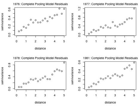
Fig. 6 Semivariograms by year for complete pooling model residuals
Observe that each panel shows an increasing semivariance with distance that doesn't appear to level off. This is indicative of a non-stationary process, one in which the mean and variance are changing with distance. Nest I repeat these steps for the random intercepts model.
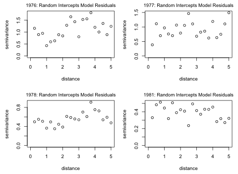
Fig. 7 Semivariograms by year for random intercepts model residuals
It's pretty clear that while there was serious spatial correlation among the residuals in the complete pooling model of Problem 1 (as evidenced by the clear increasing trend in the semivariogram plot), this has more or less disappeared in the residuals of the random intercepts model. In Fig. 7 there appears to be only random scatter with no clear trend except perhaps for a slight trend in the years 1976 and 1978. Thus by accounting for the hierarchical nature of the data using a mixed effects model we may have also managed to account for much of the spatial correlation.
A formal test of spatial correlation is the Mantel test. The Mantel correlation for this problem is the Pearson correlation of the distance between pairs of residuals and the geographic distance between pairs of lakes. The null distribution is obtained by randomly permuting the residuals among the lakes. We can't do the permutation to all of the residuals simultaneously because that would disrupt both their temporal and their spatial relationships. To do this correctly we would need to permute each four year block of residuals at each lake as a unit to keep their temporal patterns intact. Alternatively we can carry out the Mantel test separately by year. I write a function that selects the appropriate observations by year and carries out the Mantel test for that year.
The Mantel test indicates that there is a significant residual spatial correlation in 1978.
Given that the Mantel test is only just significant and the fact that we've had some success in reducing spatial correlation by including random intercepts in the model (which are necessarily spatially referenced since we have one per lake), an obvious choice is to include latitude and longitude in the model. We can just add them as predictors, add them as a response surface, or add them as smooths. I try both an additive smooth of latitude and longitude as well as a symmetrical two-dimensional smooth.
All of the models that include latitude and longitude improve on the random intercepts model. I extract the Pearson residuals from each model and carry out the Mantel test. To facilitate doing this repeatedly I organize everything as a function.
Now none of the correlations are statistically significant. Any of the models that include latitude and longitude will work here.
| Jack Weiss Phone: (919) 962-5930 E-Mail: jack_weiss@unc.edu Address: Curriculum for the Environment and Ecology, Box 3275, University of North Carolina, Chapel Hill, 27599 Copyright © 2012 Last Revised--May 2, 2012 URL: https://sakai.unc.edu/access/content/group/2842013b-58f5-4453-aa8d-3e01bacbfc3d/public/Ecol562_Spring2012/docs/solutions/finalpart1.htm |