Formula:
O3 ~ s(vh) + s(wind) + s(humidity) + s(temp) + s(ibh) + s(dpg) +
s(ibt) + s(vis) + s(day)
Parametric coefficients:
Estimate Std. Error t value Pr(>|t|)
(Intercept) 11.776 0.198 59.3 <2e-16 ***
---
Signif. codes: 0 ‘***’ 0.001 ‘**’ 0.01 ‘*’ 0.05 ‘.’ 0.1 ‘ ’ 1
Approximate significance of smooth terms:
edf Ref.df F p-value
s(vh) 1.00 1.00 8.51 0.00380 **
s(wind) 1.00 1.00 5.29 0.02214 *
s(humidity) 3.60 4.48 2.78 0.02220 *
s(temp) 4.80 5.88 5.03 7.0e-05 ***
s(ibh) 3.03 3.71 1.28 0.27957
s(dpg) 3.23 4.11 10.74 2.6e-08 ***
s(ibt) 1.84 2.37 1.37 0.25636
s(vis) 2.26 2.82 6.26 0.00053 ***
s(day) 3.98 5.01 16.13 3.8e-14 ***
---
Signif. codes: 0 ‘***’ 0.001 ‘**’ 0.01 ‘*’ 0.05 ‘.’ 0.1 ‘ ’ 1
R-sq.(adj) = 0.797 Deviance explained = 81.3%
GCV score = 14.099 Scale est. = 12.998 n = 330
There are four models to consider. Each of these models contains all the other smooths but they differ in whether s(ibh) and s(ibt) are present.
I refit the first model using maximum likelihood.
Family: gaussian
Link function: identity
Formula:
O3 ~ s(vh) + s(wind) + s(humidity) + s(temp) + s(ibh) + s(dpg) +
s(ibt) + s(vis) + s(day)
Parametric coefficients:
Estimate Std. Error t value Pr(>|t|)
(Intercept) 11.776 0.201 58.7 <2e-16 ***
---
Signif. codes: 0 ‘***’ 0.001 ‘**’ 0.01 ‘*’ 0.05 ‘.’ 0.1 ‘ ’ 1
Approximate significance of smooth terms:
edf Ref.df F p-value
s(vh) 1.00 1.00 10.27 0.00149 **
s(wind) 1.00 1.00 4.57 0.03325 *
s(humidity) 1.00 1.00 10.68 0.00120 **
s(temp) 4.12 5.12 9.13 3.0e-08 ***
s(ibh) 1.00 1.00 0.01 0.93549
s(dpg) 3.70 4.68 9.70 3.0e-08 ***
s(ibt) 1.00 1.00 2.19 0.14025
s(vis) 2.03 2.54 6.76 0.00047 ***
s(day) 4.75 5.90 14.51 2.1e-14 ***
---
Signif. codes: 0 ‘***’ 0.001 ‘**’ 0.01 ‘*’ 0.05 ‘.’ 0.1 ‘ ’ 1
R-sq.(adj) = 0.793 Deviance explained = 80.5%
ML score = 910.51 Scale est. = 13.297 n = 330
The p-values have changed but neither s(ibh) and s(ibt) yield statistically significant Wald tests.
I fit the remaining three models by dropping terms from this model.
There are a number of ways to proceed. We can start with both terms in the model and try to drop one of them. This is what the Wald tests are reporting.
Model 1: O3 ~ s(vh) + s(wind) + s(humidity) + s(temp) + s(ibh) + s(dpg) +
s(vis) + s(day)
Model 2: O3 ~ s(vh) + s(wind) + s(humidity) + s(temp) + s(ibh) + s(dpg) +
s(ibt) + s(vis) + s(day)
Resid. Df Resid. Dev Df Deviance F Pr(>F)
1 310.4 4143
2 309.4 4114 1.011 28.98 2.155 0.143
Model 1: O3 ~ s(vh) + s(wind) + s(humidity) + s(temp) + s(dpg) + s(ibt) +
s(vis) + s(day)
Model 2: O3 ~ s(vh) + s(wind) + s(humidity) + s(temp) + s(ibh) + s(dpg) +
s(ibt) + s(vis) + s(day)
Resid. Df Resid. Dev Df Deviance F Pr(>F)
1 310.4 4115
2 309.4 4114 0.9878 0.8801 0.067 0.793
Both of these tests agree with the Wald tests. The tests say that we can legitimately drop either smooth given that the other is present in the model. Under each scenario we can then try to drop the remaining smooth.
Model 1: O3 ~ s(vh) + s(wind) + s(humidity) + s(temp) + s(dpg) + s(vis) +
s(day)
Model 2: O3 ~ s(vh) + s(wind) + s(humidity) + s(temp) + s(ibh) + s(dpg) +
s(vis) + s(day)
Resid. Df Resid. Dev Df Deviance F Pr(>F)
1 310.9 4154
2 310.4 4143 0.537 10.84 1.512 0.198
So having dropped s(ibt) we can now also drop s(ibt).
Model 1: O3 ~ s(vh) + s(wind) + s(humidity) + s(temp) + s(dpg) + s(vis) +
s(day)
Model 2: O3 ~ s(vh) + s(wind) + s(humidity) + s(temp) + s(dpg) + s(ibt) +
s(vis) + s(day)
Resid. Df Resid. Dev Df Deviance F Pr(>F)
1 310.9 4154
2 310.4 4115 0.5603 38.94 5.242 0.0408 *
---
Signif. codes: 0 ‘***’ 0.001 ‘**’ 0.01 ‘*’ 0.05 ‘.’ 0.1 ‘ ’ 1
This test tells us that having dropped s(ibh) we should not drop s(ibt). When s(ibt) is in the model without s(ibh), s(ibt) is statistically significant. Finally we could try to drop both terms simultaneously.
Model 1: O3 ~ s(vh) + s(wind) + s(humidity) + s(temp) + s(dpg) + s(vis) +
s(day)
Model 2: O3 ~ s(vh) + s(wind) + s(humidity) + s(temp) + s(ibh) + s(dpg) +
s(ibt) + s(vis) + s(day)
Resid. Df Resid. Dev Df Deviance F Pr(>F)
1 310.9 4154
2 309.4 4114 1.548 39.82 1.934 0.156
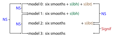
According to this test we could drop s(ibh) and s(ibt) together. Fig. 1 summarizes the different model comparisons we've made.
Fig. 1 Model comparisons involving s(ibt) and s(ibh)
The results of the partial F-tests are fairly clear. If you start with neither variable in the model model 3 in Fig. 1), then the partial F-test says you should add s(ibt) but not s(ibh). If you start with both variables in the model (model 0 in Fig. 1) then the partial F-test says you can drop either one. If you drop s(ibh) first then the partial F-test says you should not drop s(ibt). It’s only in the case when you choose to drop s(ibt) first that the partial F-test tells you to drop s(ibh) too and end up with neither. That’s why stepwise methods typically use forward and backward selection in selecting variables to deal exactly with this scenario.
So what should we conclude? Clearly the terms s(ibh) and s(ibt) are correlated and their presence together in a model is influencing the significance test of the other. The tests of either one in isolation, separated from the other, are more honest tests and tell us that we should retain s(ibt) but drop s(ibh). This conclusion is confirmed if we compare the four models using AIC.
Thus we should retain s(ibt) and drop s(ibh).
I refit the model without s(ibh) and plot the smooths.
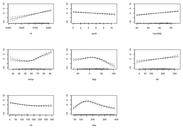
Fig. 2 Partial response functions corresponding to the seven smoother terms
We can obtain the estimated degrees of freedom for these smooths from the summary table of the model.
Formula:
O3 ~ s(vh) + s(wind) + s(humidity) + s(temp) + s(dpg) + s(ibt) +
s(vis) + s(day)
Parametric coefficients:
Estimate Std. Error t value Pr(>|t|)
(Intercept) 11.8 0.2 58.8 <2e-16 ***
---
Signif. codes: 0 ‘***’ 0.001 ‘**’ 0.01 ‘*’ 0.05 ‘.’ 0.1 ‘ ’ 1
Approximate significance of smooth terms:
edf Ref.df F p-value
s(vh) 1.00 1.00 10.74 0.00117 **
s(wind) 1.00 1.00 4.64 0.03192 *
s(humidity) 1.00 1.00 10.73 0.00117 **
s(temp) 4.12 5.12 9.80 7.4e-09 ***
s(dpg) 3.70 4.68 9.81 2.5e-08 ***
s(ibt) 1.00 1.00 5.13 0.02419 *
s(vis) 2.03 2.54 6.80 0.00045 ***
s(day) 4.76 5.91 15.16 4.7e-15 ***
---
Signif. codes: 0 ‘***’ 0.001 ‘**’ 0.01 ‘*’ 0.05 ‘.’ 0.1 ‘ ’ 1
R-sq.(adj) = 0.793 Deviance explained = 80.5%
ML score = 910.52 Scale est. = 13.258 n = 330
From the graph and the summary output, the smooths of vh, wind, humidity, and ibt are roughly linear. I refit the model with these as linear terms.
Fig. 3 displays plots of the partial response functions for the remaining smooths.
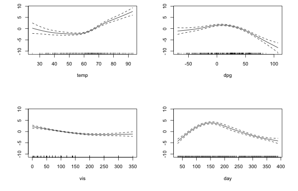
Fig. 3 Partial response functions for the four remaining smooths
Each graph is too asymmetric to be a quadratic but we could try replacing the smooths with a breakpoint regression model consisting of two connected line segments with different slopes. To proceed we need to obtain an estimate for the location of the breakpoints. By inspecting the graphs we can obtain a reasonable range of values over which to search. The code below carries out the search for each smooth separately. In each case we keep the rest of the model the same but replace one smooth with a breakpoint model. So, in each case I replace the given s(x) with x + I((x-c)*(x>c)).
Table 1 summarizes the results of the search.
| Table 1 Breakpoint model results |
| Variable | Range examined | Estimated breakpoint | Reported AIC | Actual AIC |
temp |
(40, 70) |
60 |
1809.20 |
1811.20 |
dpg |
(–10, 40) |
16 |
1808.91 |
1810.91 |
vis |
(100, 250) |
200 |
1808.78 |
1810.78 |
day |
(100, 200) |
144 |
1807.12 |
1809.12 |
The AIC values returned by the AIC function on each of the breakpoint models underestimates the number of parameters by 1 because it doesn't count the breakpoint parameter that we estimated by hand. Thus we need to add 2 to each of the AIC values because AIC = –2*log-likelihood + 2k, where k is the number of parameters. I recalculate the AIC and add to the list the AIC of the model that contains all four of the smooths.
The AIC values of the breakpoint models exceed that of the four-smooth model except for the breakpoint model involving day. Thus we can legitimately argue that only s(day) should be replaced with a breakpoint model.
Method 1
I start by plotting the smooth of day. To obtain just this smooth I plot the gam object and use the select argument to select the fourth smooth.
To add the breakpoint model to this graph we need to know where to start it. The first value of day in the data set is 33.
To figure out what the y-coordinate of the smooth is at day = 33, I experiment by adding points to the graph with the points function. After trying a number of values near –5, I settle on –4.3. Fig. 4 shows the graph of the smooth with this point plotted.
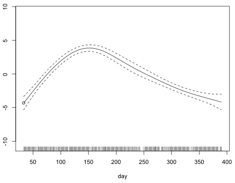
Fig. 4 Graph of s(day) with left-hand endpoint of the curve selected
Next I write a function for the breakpoint model. The coefficients of the breakpoint terms are entries 6 and 7 of the coefficients vector.
The breakpoint function is the following.
If we evaluate the breakpoint function at day = 33 we don't get –4.3.
We need to add a constant to the breakpoint model so that we get –4.3 at day = 33. The amount we need is –6.96544.
I rewrite the breakpoint function adding this constant to the expression and use the curve function to add the breakpoint function for day to the graph of the smooth.
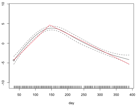
Fig. 5 Graph of s(day) along with the breakpoint model using Method 1
Method 2
A simpler method is to use the shift argument of plot.gam (the plot method for gam objects) and to specify for this argument the parametric portion of the gam model with all predictors set to their mean values.
For the breakpoint function we do the same thing.
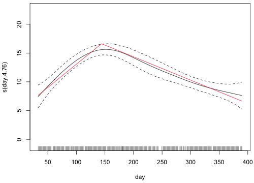
Fig. 6 Graph of s(day) along with the breakpoint model using Method 2
| Jack Weiss Phone: (919) 962-5930 E-Mail: jack_weiss@unc.edu Address: Curriculum for the Environment and Ecology, Box 3275, University of North Carolina, Chapel Hill, 27599 Copyright © 2012 Last Revised--March 27, 2012 URL: https://sakai.unc.edu/access/content/group/2842013b-58f5-4453-aa8d-3e01bacbfc3d/public/Ecol562_Spring2012/docs/solutions/assign9.htm |