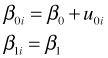
The important characteristic of these data is that we have multiple measurements from the same plant (5 values per plant) as well as measurements made on different plants. Thus the data are heterogeneous. We can account for this by fitting a mixed effects model in which plant is identified as the grouping variable. Preliminary plots indicate that growth is nearly linear over the time period in question so a linear regression of root versus week treating week as a continuous variable makes sense here. Letting i denote the plant and j the observation on that plant we have
![]()
where ![]() . With only 12 plants it will be overkill to try to let both the intercepts and slopes be random. In fact as we'll see, except for an effect due to fertilizer, the slopes show almost no variability across plants. A minimal mixed effects model is a random intercepts model in which the intercepts are allowed to vary across plants but the slopes are treated as constant.
. With only 12 plants it will be overkill to try to let both the intercepts and slopes be random. In fact as we'll see, except for an effect due to fertilizer, the slopes show almost no variability across plants. A minimal mixed effects model is a random intercepts model in which the intercepts are allowed to vary across plants but the slopes are treated as constant.
where ![]() . This model is fit as follows.
. This model is fit as follows.
The linear relationship between root size and time is highly significant.
Fertilizer is a level-2 variable. It was randomly applied to whole plants, not to the individual times at which a plant was measured. As a level-2 variable fertilizer can affect the level-2 equation either by modifying the intercept, the slope, or both. We consider each possibility in turn.
The model in which fertilizer affects both the intercepts and slopes ranks best. We carry out a formal significance test of the individual terms.
There is a significant interaction between week and fertilizer (the slope effect) as well as a significant effect of fertilizer on the intercepts.
I display the autocorrelation function of the residuals using a Bonferroni correction for four tests (corresponding to the four lags shown). None of the spikes achieves statistical significance so there is no need to consider a correlation model for the residuals.
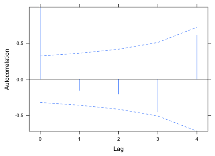 |
Fig. 1 ACF for the level-1 residuals |
I color the lines and points to indicate if fertilizer is present (red) or absent (blue).
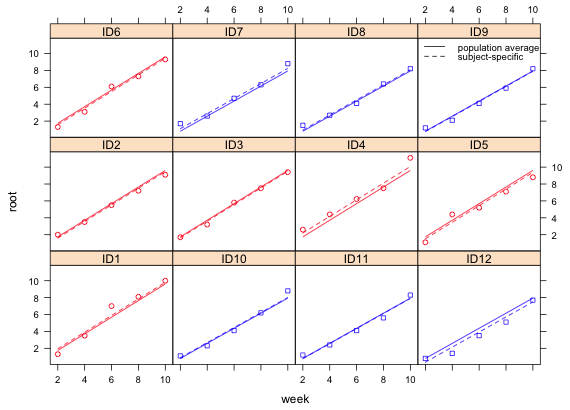 |
Fig. 2 Plot of fitted model: population average (consisting of estimates of the fixed effects only) and subject specific (consisting of estimates of the fixed effects and predictions of the random effects) along with the data. The data are colored red (fertilizer added) and blue (fertilizer absent). |
In Fig. 2 we see that a regression line whose slope varies only by fertilizer type seems to provide a reasonable fit to the data. There is no need for each plant to have its own slope. If one tries to fit a random slopes and intercepts model, the following message is obtained.
It is possible by adjusting various control parameters to get a slopes and intercept model to converge here. The lme function has a control argument for which one can use the lmeControl function to modify the default settings of the optimization algorithm. In the run below I change the optimization function from the default nlminb to optim and increase the maximum number of iterations for various steps.
Notice that before including fertilizer in the model, a random slopes and intercepts model has a lower AIC than a random intercepts model, but once fertilizer is included as a predictor of the slopes there is no longer a need for the random slopes. Fitting the random slopes and intercepts model in this case increases the AIC over a random intercepts model.
These data consist of a random sample of farms and then multiple measurements taken from the same farm. To investigate whether this structure matters we can fit a random intercepts model in which there are no predictors, just an intercept, and in which we allow that intercept to vary across farms.
From the output we see that the variance within farms, σ2, is 5.97 while the variance between between farms, τ2, is 66.95 indicating that the variability of the response between farms is 11 times its variability within farms.
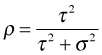
The intra-class correlation compares the variability between farms to the total variability (sum of the variability between and within farms).
I fit a random intercepts mode in which nitrogen is a level-1 predictor of size.
Random effects:
Formula: ~1 | farm
(Intercept) Residual
StdDev: 8.316789 1.920269
Fixed effects: size ~ N
Value Std.Error DF t-value p-value
(Intercept) 85.58120 2.5276865 95 33.85752 0
N 0.70806 0.0931177 95 7.60392 0
Correlation:
(Intr)
N -0.732
Standardized Within-Group Residuals:
Min Q1 Med Q3 Max
-2.80413111 -0.63410087 0.02949117 0.70724199 2.19176486
Number of Observations: 120
Number of Groups: 24
Like the model in Part 1, in order to fit a random slopes and intercepts model here it is necessary to adjust the default optimization settings of the lme function. If we do so we fail to find evidence that both slopes and intercepts should be random. The AIC of this model is higher than the comparable random intercepts model.
| Jack Weiss Phone: (919) 962-5930 E-Mail: jack_weiss@unc.edu Address: Curriculum for the Environment and Ecology, Box 3275, University of North Carolina, Chapel Hill, 27599 Copyright © 2012 Last Revised--March 13, 2012 URL: https://sakai.unc.edu/access/content/group/2842013b-58f5-4453-aa8d-3e01bacbfc3d/public/Ecol562_Spring2012/docs/solutions/assign7.htm |