Assignment 6—Solution

Question 1

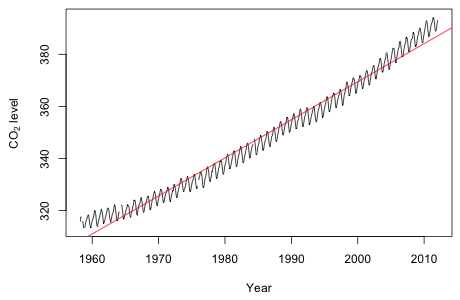
Fig. 1  Raw data plus linear trend model

The plot shows a marked deviation from linearity.

Question 2

Model 1: average ~ decimal.date
Model 2: average ~ decimal.date + I(decimal.date^2)
  Res.Df    RSS Df Sum of Sq      F    Pr(>F)   
1    638 7284.0                                 
2    637 3051.4  1    4232.5 883.57 < 2.2e-16 ***
---
Signif. codes:  0 ‘***’ 0.001 ‘**’ 0.01 ‘*’ 0.05 ‘.’ 0.1 ‘ ’ 1

The quadratic term is highly significant.

Question 3

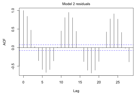Fig. 2  ACF for the model 2 residuals

The plot shows an obvious cycle at 12 months (the point at which the graph begins to repeat itself).

Question 4

Model 1: average ~ decimal.date + I(decimal.date^2)
Model 2: average ~ decimal.date + I(decimal.date^2) + sin(2 * pi/12 *
    ID) + cos(2 * pi/12 * ID)
  Res.Df     RSS Df Sum of Sq      F    Pr(>F)   
1    637 3051.41                                 
2    635  532.88  2    2518.5 1500.6 < 2.2e-16 ***
---
Signif. codes:  0 ‘***’ 0.001 ‘**’ 0.01 ‘*’ 0.05 ‘.’ 0.1 ‘ ’ 1

The addition of the trigonometric terms of period 12 is highly significant.

Question 5

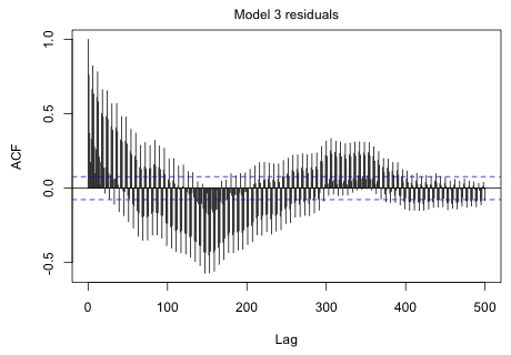Fig. 3  ACF for the model 3 residuals

Although things are damping down with time, it's pretty clear we have a cycle somewhere in excess of 300 months.

Question 6

I try fitting models with a period of 250 months up to a period of 400 months and save the AIC from each model.

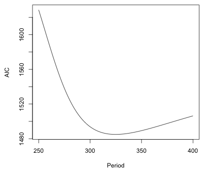Fig. 4   AIC values for different periodic models, period 250 to 400

Although a period of 325 minimizes AIC, it's pretty clear from the graph that a number of other choices for the period would do nearly as well. This is not surprising given we only have enough data to observe two full cycles.

Model 1: average ~ decimal.date + I(decimal.date^2) + sin(2 * pi/12 *
    ID) + cos(2 * pi/12 * ID)
Model 2: average ~ decimal.date + I(decimal.date^2) + sin(2 * pi/12 *
    ID) + cos(2 * pi/12 * ID) + sin(2 * pi/325 * ID) + cos(2 *
    pi/325 * ID)
  Res.Df    RSS Df Sum of Sq     F    Pr(>F)   
1    635 532.88                                
2    633 371.98  2     160.9 136.9 < 2.2e-16 ***
---
Signif. codes:  0 ‘***’ 0.001 ‘**’ 0.01 ‘*’ 0.05 ‘.’ 0.1 ‘ ’ 1

The addition of the trigonometric terms of period 325 is highly significant.

Question 7

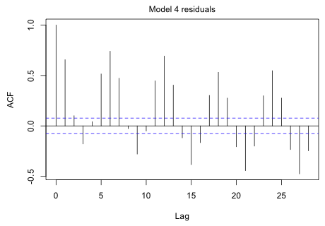Fig. 5   ACF of the model 4 residuals

The graph shows an obvious cycle at six months.

Model 1: average ~ decimal.date + I(decimal.date^2) + sin(2 * pi/12 *
    ID) + cos(2 * pi/12 * ID) + sin(2 * pi/325 * ID) + cos(2 *
    pi/325 * ID)
Model 2: average ~ decimal.date + I(decimal.date^2) + sin(2 * pi/12 *
    ID) + cos(2 * pi/12 * ID) + sin(2 * pi/325 * ID) + cos(2 *
    pi/325 * ID) + sin(2 * pi/6 * ID) + cos(2 * pi/6 * ID)
  Res.Df    RSS Df Sum of Sq      F    Pr(>F)   
1    633 371.98                                 
2    631 184.47  2    187.51 320.69 < 2.2e-16 ***
---
Signif. codes:  0 ‘***’ 0.001 ‘**’ 0.01 ‘*’ 0.05 ‘.’ 0.1 ‘ ’ 1

The addition of the trigonometric terms of period 6 is highly significant.

Question 8

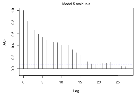Fig. 6   ACF of the model 5 residuals

The decaying pattern of the ACF is highly suggestive of an autoregressive process.

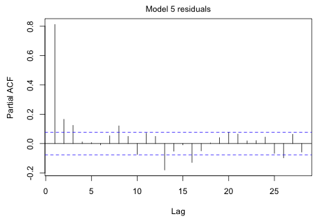Fig. 7   PACF of the model 5 residuals

The sharp spike at lag 1 in the PACF suggests that the autoregressive process may be AR(1). The fact that there are two much smaller significant spikes at lags 2 and 3 suggests we should also consider and AR(2) or AR(3). Because the drop from the first spike is sudden while the decay of spikes 2 and 3 is gradual, we might also consider adding some moving average terms.

Question 9

I start by fitting the last model using the gls function of the nlme package.

From the ACF and PACF I consider ARMA processes up to order 3. Because the PACF is a bit ambiguous, I also include moving average processes up to order 3.

We see a large drop in AIC from model5 (p=0, q=0) to an AR(1) model and then to an ARMA(1,1) model. There is no additional improvement until the last model examined, the ARMA(3,3) model, which ranks best. I refit that model as model6.

Question 10

Fig. 8a shows the ACF of the normalized residuals. There are still a number of significant spikes at various lags. We haven't been correcting for the large number of tests that we've been doing. Because we've included a period 325 term determined on the basis of examining an ACF, I feel justified in including a Bonferroni correction for 325 tests (Fig. 8b).

(a)	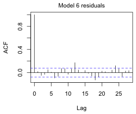(b)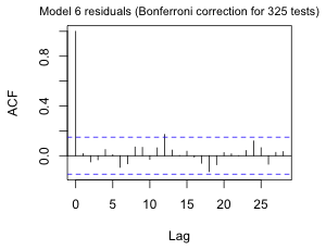
Fig. 8  ACF for the ARMA(3,3) quadratic model with three periodic terms using (a) alpha = .05 and (b) alpha = .05/325, a Bonferroni correction to account for testing at 325 different lags.

So, even with such a large Bonferroni correction there remains a significant spike at lag 12. Apparently the trig terms have not adequately accounted for the annual cycle.

Question 11

I replace the ARMA(3,3) model with an AR(12) model.

Now a fairly modest Bonferroni correction removes the significance of the spike at lag 12.

(a)	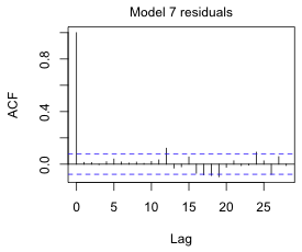(b)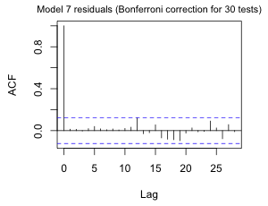
Fig. 9  ACF for the AR(12) quadratic model with three periodic terms using (a) alpha = .05 and (b) alpha = .05/30, a Bonferroni correction to account for testing at 30 different lags.

Question 12

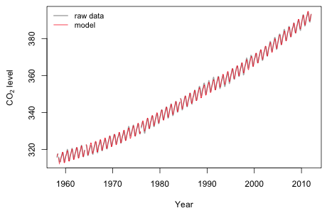Fig. 10   Plot of model predictions and the raw data

I zoom in on a the more recent portion of the plot to get a better sense of the fit.

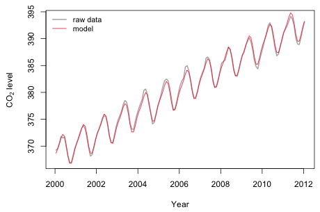Fig. 11   Plot of model predictions and the raw data for 2000 – 2012

It appears that there is a degree of irregularity to the annual cycle that we fail to match. The amplitude varies slightly over time. If we had some useful time-dependent predictors we might be able to explain this deviation from a purely sinusoidal pattern.

The standard tool for detecting signals in time series is the periodogram (spectrum). If we examine the spectrum of the residuals of the quadratic model, the three cycles we found are seen as being the dominant cycles. (I refit the model to the interpolated data because the spectrum function does not permit missing data.) This is further justification for the model we've fit.

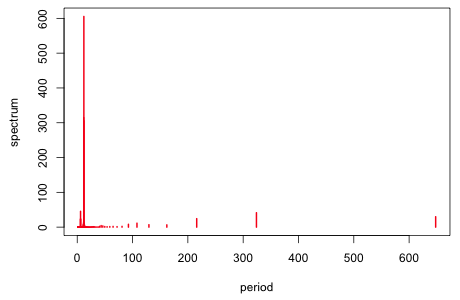Fig. 12   Spectrum of the residuals from the quadratic model

Course Home Page