Assignment 3—Solution

Question 1

I read in the data and calculate the Simpson's diversity index. The species data lie in columns 2 through 76 of the data frame so I select only those columns to calculate the diversity index.

I next recode diversity so that the current values of 1 are reassigned to zero.

Question 2

Since we previously found the best model to be the interaction model, I start there.

Response: simpson2
                 Df  Sum Sq Mean Sq F value    Pr(>F)   
factor(week)      3 1.04936 0.34979  9.9617 5.971e-05 ***
NAP               1 1.75753 1.75753 50.0537 2.253e-08 ***
factor(week):NAP  3 0.03869 0.01290  0.3673     0.777   
Residuals        37 1.29918 0.03511                     
---
Signif. codes:  0 ‘***’ 0.001 ‘**’ 0.01 ‘*’ 0.05 ‘.’ 0.1 ‘ ’ 1

We see that the interaction is not statistically significant. We also see that when week is added to a model containing NAP, the variable week is significant (p < .001). I drop the interaction term and fit the additive model. I change the order of the variables so we get a test of week in the presence of NAP, the opposite of the test given in the above table.

Response: simpson2
             Df  Sum Sq Mean Sq F value    Pr(>F)   
NAP           1 2.11324 2.11324 63.1824 9.278e-10 ***
factor(week)  3 0.69364 0.23121  6.9129 0.0007383 ***
Residuals    40 1.33787 0.03345                     
---
Signif. codes:  0 ‘***’ 0.001 ‘**’ 0.01 ‘*’ 0.05 ‘.’ 0.1 ‘ ’ 1

From this table we see that week is significant in the presence of NAP and from the previous table we know that NAP is significant in the presence of week. Thus we should retain both week and NAP in the model and report the additive model.

Question 3

The summary table is shown below.

Residuals:
     Min       1Q   Median       3Q      Max
-0.32603 -0.13247  0.01124  0.10730  0.39956

Coefficients:
              Estimate Std. Error t value Pr(>|t|)   
(Intercept)    0.60263    0.05791  10.407 6.04e-13 ***
NAP           -0.20757    0.02863  -7.249 8.46e-09 ***
factor(week)2 -0.27909    0.07646  -3.650 0.000751 ***
factor(week)3 -0.04422    0.07624  -0.580 0.565122   
factor(week)4  0.02193    0.10220   0.215 0.831216   
---
Signif. codes:  0 ‘***’ 0.001 ‘**’ 0.01 ‘*’ 0.05 ‘.’ 0.1 ‘ ’ 1

Residual standard error: 0.1829 on 40 degrees of freedom
Multiple R-squared: 0.6772,            Adjusted R-squared: 0.6449
F-statistic: 20.98 on 4 and 40 DF,  p-value: 2.193e-09

The three "factor(week)" lines in the coefficients table test whether the intercepts in weeks 2, 3, and 4 are different from the intercept in week 1. What we see is that the intercepts in weeks 1 and 2 are significantly different (p = 0.00075), but intercepts in weeks 1 and 3 are not (p = 0.565), nor are the intercepts in weeks 1 and 4 (p = 0.831).

Technically there are three additional comparisons that could be made by reordering the levels of the factor variable, but you were only asked to report what you could learn from the above single summary table.

Question 4

I recode the week variable so that it is a 0-1 variable where 1 denotes week 2 and 0 denotes the remaining weeks.

It's also possible to do the recoding without using an ifelse statement. I add 0 to the result of the Boolean expression in order to convert the TRUE-FALSE values that are returned to numeric 1-0 values.

Question 5

The dummy variables for week are shown below.

The regression equations for the models of Questions 3 and 4 are shown below.

We see that the model of Question 3 (model 5) can be reduced to the model of Question 4 (model 6) by setting β₃ = β₄ = 0. Thus the models are nested. The corresponding hypothesis test is shown below.

The anova function applied to model 5 and model 6 carries out this test. The reduced model should be entered first followed by the larger model, otherwise the degrees of freedom and sum of squares for the test are given negative values in the output table.

Model 1: simpson2 ~ NAP + factor(week2)
Model 2: simpson2 ~ NAP + factor(week)
  Res.Df    RSS Df Sum of Sq      F Pr(>F)
1     42 1.3593                          
2     40 1.3379  2  0.021419 0.3202 0.7278

We fail to reject the null hypothesis (p = 0.728) and conclude that there is insufficient evidence to claim that the intercepts in weeks 3 and 4 are different from the intercept in week 1. Consequently we should use model 6. Stated differently, we have found that the two models are not significantly different from each other. Given this result we might as well choose the simpler of the two models.

Question 6

The coefficient estimates from the final model are shown below.

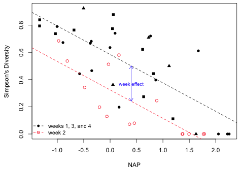
I plot the data using different symbols and symbol types for the two models. I use different symbols for the four original weeks but use different colors to denote the recoded weeks.

Fig. 1  The effect of week and NAP on Simpson's diversity. The vertical distance between the two lines is the "week effect".

Question 7

The first thing to observe is that week is not a confounder of the diversity versus NAP relationship. To demonstrate this I fit a model that contains only NAP and compare the coefficient estimate of NAP to what I obtain in a model with both NAP and week.

Observe that the coefficient of NAP is only slightly different with week in the model in model6, so week is at best only a weak confounder. That's the case here because the distributions of NAP in the two weeks are not that different.

To explain the role that week plays in the final model you need to also explain the role that NAP plays in the model. In the hint I suggested that you contrast this model, a model that has both week and NAP in it, with a model that just has week in it. If week is the variable of interest and NAP is considered a nuisance variable, then a model with only week in it is what's called an analysis of variance model (it tests for differences between the week means) whereas the current model is called an analysis of covariance model (it examines the difference in the week means while controlling for the continuous variable NAP). I compare the estimates from these two models below.

In the analysis of variance model, model0, the week effect corresponds to the difference in the mean diversities between week 2 and the remaining weeks. From the output we see that the mean in the other 3 weeks is 0.525 and the mean is week 2 is –0.300 lower than this. In the analysis of covariance model, model6, the mean diversity in week 2 is again lower than it is in the other three weeks, this time by 0.260. The difference now though is that there is no single mean diversity that is being compared across the two weeks because the mean diversity changes with NAP. The week effect instead corresponds to the vertical distance between the two regression lines shown in Fig. 1. So once we specify the value of NAP we can calculate the mean diversity in weeks 1, 3, and 4. Then to obtain the diversity in week 2 we just have to lower this value by 0.260.

The formal way of describing this is as follows. "After controlling for NAP we find that mean diversity in week 2 is 0.260 lower than it is in weeks 1, 3, and 4." Another way to say this is the following. "After adjusting for the effect of NAP, mean diversity in week 2 is 0.260 lower than it is in weeks 1, 3, and 4."

Course Home Page