Assignment 10—Solution

Question 1

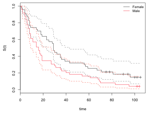
Fig. 1  Survivor curves separately by sex of flower. Point estimate and 95% confidence intervals are shown. Here the survivor curve represents the probability that the waiting time for the first insect visit exceeds the time shown.

Question 2

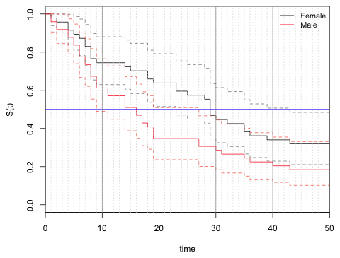
I redo the graph of Question 1 but zoom in on the time interval (0, 50). I add solid grid lines at every 10 time units and dotted grid lines at each time unit.

Fig. 2  Survivor curves and 95% confidence intervals from Fig. 1 shown with grid lines added to facilitate estimating 95% confidence intervals for the median waiting times.

From the graph we see that the horizontal line at S(t) = 0.5 (the median) intersects the male 95% confidence bands at 9 and 27. It intersects the female 95% confidence bands at 23 and 43.

Alternatively, the print function has a method for survfit objects. When print is applied to a survfit object it returns the median and 95% confidence intervals of the median.

   Non-visible functions are asterisked

      records n.max n.start events median 0.95LCL 0.95UCL
sex=F      47    47      47     39     29      23      43
sex=M      49    49      49     47     16       9      27

Question 3

We can test for differences in survivorship by sex with the log rank test.

N Observed Expected (O-E)^2/E (O-E)^2/V
sex=F 47 39 49.46 2.213 5.453
sex=M 49 47 36.54 2.996 5.453

Chisq= 5.5 on 1 degrees of freedom, p= 0.01953

The default test is the standard log rank test with equally weighted waiting times (rho = 0). We see that the flower sexes differ significantly in time to the first insect visit. We can redo the test but weight the early waiting times more than later weighting times (rho = 1).

N Observed Expected (O-E)^2/E (O-E)^2/V
sex=F 47 20.43 26.81 1.520 5.094
sex=M 49 28.32 21.93 1.858 5.094

Chisq= 5.1 on 1 degrees of freedom, p= 0.02401

The results are the same. Female flowers wait longer to be visited by insects than do male flowers.

Question 4

To obtain the hazard ratio I fit a proportional hazards model for survival time with sex as the only predictor.

  n= 96, number of events= 86

        coef exp(coef) se(coef)      z Pr(>|z|) 
sexM 0.50216   1.65228  0.21813 2.3021  0.02133 *
---
Signif. codes:  0 ‘***’ 0.001 ‘**’ 0.01 ‘*’ 0.05 ‘.’ 0.1 ‘ ’ 1

     exp(coef) exp(-coef) lower .95 upper .95
sexM    1.6523    0.60522    1.0775    2.5337

Concordance= 0.569  (se = 0.031 )
Rsquare= 0.054   (max possible= 0.999 )
Likelihood ratio test= 5.33  on 1 df,   p=0.020994
Wald test            = 5.3  on 1 df,   p=0.021328
Score (logrank) test = 5.41  on 1 df,   p=0.020051

Females are the reference group thus the coefficient of sex is the effect on the log hazard of being male relative to being female. Formally we have the following

Exponentiating these equations we obtain the hazards for males and females.

This yields the following hazard ratio for males versus females.

From the output this hazard ratio is estimated to be 1.65. The hazard ratio is a ratio of these rates. The hazard itself is a probability rate and can be use to infer the expected number of events per unit time. So, we can say any of the following.

1. In a given time period unvisited male flowers can expect 1.65 times as many visitations by insects as unvisited female flowers.
2. A female flower waits 1.65 times as long as a male flower for the first insect visit.
3. At any instant the risk of an unvisited male flower being visited by an insect is 1.65 times the risk of an unvisited female flower being visited by an insect.
4. In any period of time, male flowers are 1.65 times as likely to be visited as female flowers.
5. Male flowers are being visited at 1.65 times the rate that female flowers are being visited.

Question 5

The proportional hazards assumption says that the hazard function can be decomposed into a product of two components one that depends upon time and another that depends upon predictors but not time.

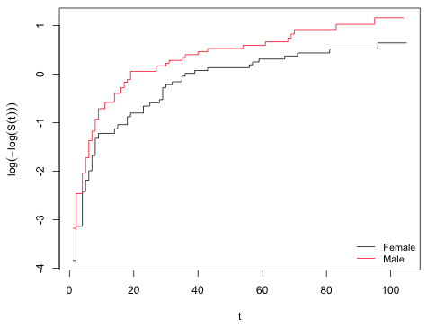
A graphical test of the proportional hazards function for a categorical predictor like sex, is to plot log(log(–S(t)) against time (t) separately for each sex and see if the graphs are roughly parallel.

Fig. 3  Graphical assessment of the proportional hazards function. As we can see the log(-log(S(t)) curves are parallel over most of the survival times.

The graphs are parallel nearly their entire length. (Note: It's impossible for the curves to be parallel at the very beginning because both curves begin at the same point.) We can obtain a formal test and a second graphical test of the proportional hazards assumption by using the cox.zph function.

The test is nowhere near being statistically significant.

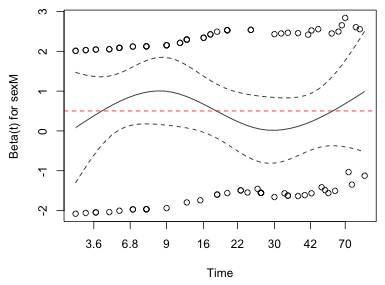
Fig. 4  Estimate of how the coefficient of sex varies over time in the proportional hazards model

If the proportional hazards assumption holds, then the regression coefficients should not depend upon time. Fig. 4 shows how the coefficient of the predictor sex changes over time. Superimposed on the graph is the estimated constant sex effect of 0.50 that was obtained from the Cox model. Although the Fig. 4 shows that the sex coefficient does change over time, the Cox estimate of 0.5 lies entirely within the displayed confidence limits. As a result we cannot reject 0.5 as a possible value for the parameter at any time and so the coefficient of sex could easily be constant.

Question 6

Scale= 1.067

Weibull distribution
Loglik(model)= -391.7   Loglik(intercept only)= -394.7
            Chisq= 5.93 on 1 degrees of freedom, p= 0.015
Number of Newton-Raphson Iterations: 5
n= 96

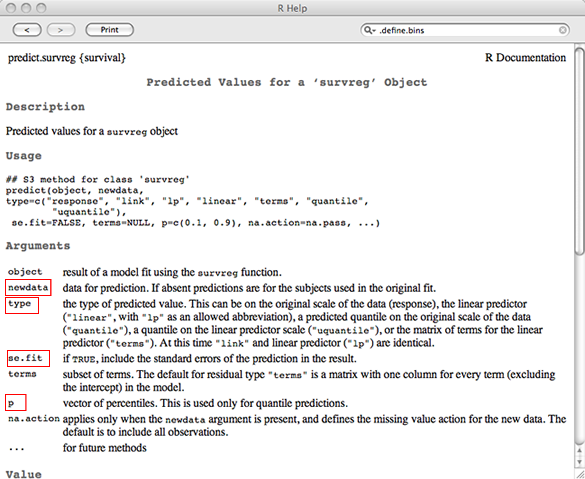
If we examine the help screen of the predict method for survreg objects we see that the arguments we need to obtain predictions of the median are newdata, type, se.fit, and p. These are highlighted in Fig. 5.

Fig. 5  Estimate of how the coefficient of sex varies over time in the proportional hazards model

To get predictions of the median we select type="quantile" and p = 0.5. To get the standard error we use se.fit=T. To obtain these estimates for males and females we need to include these values for sex in a newdata argument.

$se.fit
        1         2
3.0675624 5.6009253

Course Home Page