Assignment 1— Solution

Question 1

I read in the data and calculate the Simpson's diversity index. The species data lie in columns 2 through 76 of the data frame so I select only those columns to calculate the diversity index.

Question 2

Effect of NAP on diversity

I start by testing if Simpson's diversity index is linearly related to NAP by fitting the following model for mean diversity.

Response: simpson
          Df Sum Sq Mean Sq F value  Pr(>F) 
NAP        1 0.5072 0.50715  5.6106 0.02242 *
Residuals 43 3.8868 0.09039                 
---
Signif. codes:  0 ‘***’ 0.001 ‘**’ 0.01 ‘*’ 0.05 ‘.’ 0.1 ‘ ’ 1

The ANOVA table carries out a test of

From the reported p-value in the ANOVA table (p = 0.022) we reject the null hypothesis and conclude that the coefficient of NAP is significantly different from zero. If we examine the estimated coefficient we see that the relationship between diversity and NAP is negative.

Is week a confounder of the relationship between diversity and NAP?

I next add week to the model. I treat week as a categorical variable and represent it in the model as three dummy regressors that indicate weeks 2, 3, and 4, respectively. Week 1 serves as the reference group.

Response: simpson
             Df  Sum Sq Mean Sq F value   Pr(>F)   
NAP           1 0.50715 0.50715  8.5782 0.005593 **
factor(week)  3 1.52201 0.50734  8.5813 0.000161 ***
Residuals    40 2.36484 0.05912                    
---
Signif. codes:  0 ‘***’ 0.001 ‘**’ 0.01 ‘*’ 0.05 ‘.’ 0.1 ‘ ’ 1

The middle line of the ANOVA table carries out a test of

From the reported p-value in the ANOVA table (p < 0.001) we reject the null hypothesis and conclude that after controlling for NAP, diversity still varies by week. If we compare the coefficient of NAP in this model with the coefficient of NAP in the model without week, we see that the coefficient has barely changed: –0.098 (with week) versus –0.108 (without week).

Given such a trivial change in the coefficient of NAP we conclude that although week is a statistically significant predictor of Simpson diversity, it is not a confounder of NAP. We obtain roughly the same estimate of the relationship between diversity and NAP whether we include week in the model or not.

We can assess this more formally by constructing a confidence interval for the coefficient of NAP in the NAP-only model.

The 95% confidence interval of the slope in the model containing only NAP is (–0.200, –0.016). Observe that when we add week to the model the estimated slope changes to –0.098, a value that lies entirely within this 95% confidence interval. Consequently we would not declare the coefficients of NAP in these two models to be significantly different from each other.

Do week and NAP interact in their effects on diversity?

Technically we should address interaction before we consider confounding. The interaction model is the following.

Response: simpson
                 Df  Sum Sq Mean Sq F value    Pr(>F)   
NAP               1 0.50715 0.50715 10.1683  0.002906 **
factor(week)      3 1.52201 0.50734 10.1720 5.045e-05 ***
NAP:factor(week)  3 0.51943 0.17314  3.4715  0.025599 * 
Residuals        37 1.84541 0.04988                     
---
Signif. codes:  0 ‘***’ 0.001 ‘**’ 0.01 ‘*’ 0.05 ‘.’ 0.1 ‘ ’ 1

The third line of the ANOVA table carries out a test of

Because the reported p-value (.026) is less than .05, we conclude that NAP and week do interact. Apparently the nature of the relationship between diversity and NAP changes depending on the week. This also means the question of confounding is irrelevant here.

Question 3

Having concluded that there is a significant interaction between week and NAP, I graph that model. In the interaction model there is a separate linear relationship between diversity and NAP in each week. I first graph the model using base graphics and then using lattice (although only one of these plots is required here).

Fig. 1   Plot of the interaction model using base graphics

The three sites with diversity = 1 in weeks 3 and 4 clearly look anomalous. In fact they are. These three sites are ones in which no animals were collected at all, yet the diversity function of the vegan package has assigned them a Simpson's diversity of 1! This would appear to be a bug.

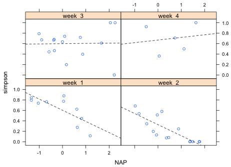
Fig. 2   Plot of the interaction model using lattice

Using the graphs the nature of the interaction between NAP and week is clear. In weeks 1 and 2 diversity has a negative relationship with NAP, but in weeks 3 and 4 there is no relationship between diversity and NAP (week 3) or at best a weakly positive one (week 4). It appears though that these last two relationships are being driven perhaps entirely by the three anomalous diversity values of 1.

Course Home Page