 possible one-stage cluster samples of size 3.
Stratified random sampling is appropriate when the population of interest consists of coherent subpopulations. In stratified random sampling we treat the subpopulations as separate populations in their own right for sampling purposes and we call the subpopulations strata. The point estimates and their precisions for the individual strata are then reassembled to form a stratified estimate of the mean and variance.
For stratified random sampling to be effective, the strata should be individually more homogeneous than the population as a whole. We want most of the variability to lie between strata rather than within strata. In ecology strata are often chosen to be habitat types. If an area exhibits an environmental gradient that is likely to have an effect on the variable we're measuring then we should construct strata boundaries that lie perpendicular to that gradient. In this case the strata are constructs that we've invented that may or may not correspond to obvious subpopulations in the field. The primary advantage of stratified random sampling is that the standard errors of our estimates are decreased because the variability that exists between the strata has been eliminated from the analysis.
Within the strata any other possible sampling scheme is legitimate. Thus we can have stratified simple random samples, stratified systematic random samples, or stratified cluster random samples. The one practical issue that needs to be decided is how to allocate resources when sampling the different strata. Proportional allocation is a logical and relatively simple approach. Stratified random sampling nearly always results in a gain in precision unless the researcher is totally clueless about his/her study subjects.
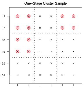
Suppose the tract occupied by our schematic population is crisscrossed by roads that provide easy access to groups of units (Fig. 1). Logistically it makes sense to sample these units as a group. Groups of sampling units that exist for reasons unrelated to the variable of interest are called clusters. If we take a random sample of clusters and then take all members of the selected clusters for our sample we've created what's called a one-stage cluster sample. Because each cluster contains four elements, to obtain a one-stage cluster sample of size 12 we need only select three clusters. Because there are nine clusters total it follows that there are possible one-stage cluster samples of size 3.
choose(9,3)
[1] 84
Using the sample function in R we can obtain a list of the clusters for our one-stage cluster sample as follows.
sample(1:9, 3, replace=FALSE)
An example of a one-stage cluster sample taken from our schematic population is shown in Fig. 1.
 |
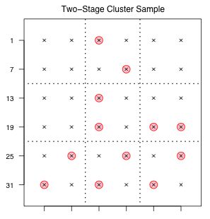 |
Fig. 1 One-stage cluster sample |
Fig. 2 Two-stage cluster sample |
A two-stage cluster sample is an extension of a one-stage cluster sample in that it adds a second sampling stage. After selecting the clusters (primary sample units) we then choose a subsample of units from each cluster (secondary sample units), generally using simple random sampling. To obtain a sample of size 12 from our schematic population using a two-stage cluster sample, we could select six clusters at the first stage and then two units from each of those clusters at the second stage. (Other possibilities are to select four primary units followed by three secondary units from each, etc.) There are  different cluster samples of this type.
choose(9,6)*(choose(4,2))^6
[1] 3919104
Using R we obtain the six primary sampling units as follows.
sample(1:9, 6, replace = FALSE)
Then if we think of the units in each cluster as being numbered 1, 2, 3, and 4 in some order, we can obtain the secondary units as follows.
sapply(1:6, function(x) sample(1:4, 2, replace=F))
[,1] [,2] [,3] [,4] [,5] [,6]
[1,] 1 3 4 3 2 2
[2,] 4 1 3 2 3 3
An example of one such two-stage cluster sample is shown in Fig. 2.
Cluster samples are often not chosen by design but are a product of circumstances. If the primary sampling unit is a quadrat or a sampling device (like a dip net or a bucket), but the object of interest is the individual of which many are found in each primary sampling unit, then a cluster sample has been obtained. Cluster samples are identified by the number of stages that are present.
Cluster sampling tends to work best when the individual clusters are as diverse as possible, at least as diverse as the population as a whole. Typically this will not be the case because cluster elements tend to be positively correlated and hence less diverse than the population as a whole. As a result parameter estimates obtained using cluster samples tend to be less precise (more variable) than estimates obtained from simple random sampling.
An advantage of cluster sampling is that a sample frame is not needed for the whole population, only for the clusters that happen to be included in the sample, and if we're doing only a one-stage cluster sample, then not even that. For a one-stage cluster sample our sample frame is just a list of the clusters. In environmental science clusters tend to be spatial or temporal units.
Stratified random samples and cluster samples are easy to distinguish after the fact, but perhaps less so before sampling begins. It's conceivable that one person's strata might be another person's clusters.
Stratified random sample |
Cluster sample |
|
|
|
|
|
|
|
|
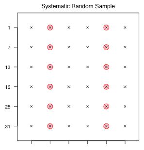
Fig. 3 Systematic sample
Systematic samples are very popular because they are very easy to carry out and are often logistically attractive. Unfortunately they have a number of problems statistically. After a random starting point in the sample frame, a systematic sample selects additional sample units at regular intervals. Thus for a systematic sample to be feasible it must be possible to order the sampling units in some way.
To obtain a systematic sample of size 12 from our schematic population of size 36, we randomly choose a value from 1, 2, or 3 as a starting place and then select every third value from that starting point until we cycle through the population. Observe that in this instance there are only three possible starting points and hence only three possible systematic samples of size 12 from this population.
Using R we obtain our systematic sample as follows.
seq(sample(1:3,1),36,3)
[1] 2 5 8 11 14 17 20 23 26 29 32 35
Fig. 3 illustrates one such sample. While the regularity of the sample may be a bit disconcerting, such a sample can be either very good or very bad.
Besides its goodness or badness, the real difficulty with systematic samples is in trying to come up with an honest measure of sampling variability. To accomplish this often requires making some rather extreme assumptions or carrying out some ad hoc statistical gymnastics.
A systematic sample is an ordered sample. The implicit assumption in systematic sampling is that it is possible to order the target area in some way and to use that order to pick a sample. Means obtained with a systematic sample of size n will be unbiased for the population mean (equal to the population mean on average) if the sample is spread out over the population in equal increments in such a way that ![]() is an integer, where N is the population size.
is an integer, where N is the population size.
Generally speaking, if the target area is large and the sampling area is small, there are no particular statistical problems inherent in using a systematic sample instead of a simple random sample. An example of such a situation would be taking a transect along an ocean bottom stopping every kilometer or so to take a sample.
How should one obtain the variance of systematic sample estimates?
If a population exhibits a trend then a judiciously selected systematic sample can be more precise than a simple random sample of the same size.
There exist formulas for calculating simple statistics and their standard errors for most of the standard sampling designs. But when sampling protocols are complicated it becomes necessary to approximate things numerically either using available software or by writing your own routines. The survey package in R can provide sample estimates along with their standard errors for all of the standard sample designs plus many additional ones. The survey package is not part of the standard R installation. So the first time you plan to use it you first need to obtain this package from the R web site.
The survey package was written by Thomas Lumley of the University of Washington, Lumley (2007), and he has provided a number of useful references for his package.
To illustrate its capabilities I use it to analyze data collected with a one-stage cluster sample. The data file is Surinam.csv, a comma-delimited file with the variable names in the first row of the file. The data are a complete inventory of all the trees in a 60 ha section of forest in Surinam. It is taken from Schreuder et al. (2004) who use it to illustrate applications of survey sampling theory to forestry.
The variable SubPlot records the subplot in which a tree occurred. There are 60 subplots identified by a combination of letter and number.
SubPlot is a factor variable in R, as indicated by the comment at the end of the unique output above "60 levels: A1 A10" etc. A factor level has both a name (the name of the subplot in this case) and a number (a number from 1 to 60). We can take advantage of the numeric values to color the subplots geographically. In the plot command below I use the numeric level of the factor levels as the value of the col= argument. Because there are only 8 numeric color levels in R, the color levels are recycled and repeated for the 60 subplot values. As Fig. 4 shows the subplots are quadrats that are geographically distinct.
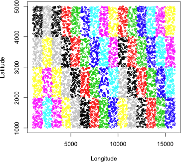 |
Fig. 4 The geographic distribution of SubPlots in the population |
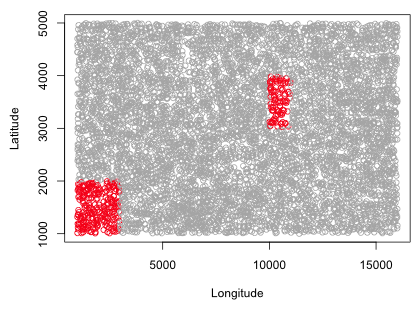
In a one-stage cluster sample we obtain a random sample of clusters and then select all the elements in that cluster. I begin by obtaining a sorted list of the unique cluster names.
Because comparisons between cluster means form the basis for the variance calculation in a one-stage cluster sample, the smallest sample size we can take that is still useful is a cluster sample with two clusters. I use the sample function to select three clusters from the list of unique clusters.
Next we need to select the elements from the population of trees that belong to clusters D2, D1, and B10. This is easily done with the Boolean intersection operator, %in%. I first illustrate its use.
So x%in%y tests whether each element in x is among the elements in y. I next obtain the one-stage cluster sample.
 |
|
|
To use the survey package we first have to define the nature of the sample using the svydesign function. For the simple sample schemes we've discussed the following four arguments are all that we need.
For id, strata, and fpc if what comes next is a variable occurring in the specified data frame then the first character in the argument must be a ~. For more complicated designs there are additional arguments that are useful. The probs argument can be used to specify the individual probabilities of selection for each element of the sample. Thus we can use the survey package to analyze any kind of sample as long as the probabilities of selection are known. The weights argument can be used instead of the probs argument (the weights are the reciprocal of the selection probabilities). In addition the weights argument can be used to handle missing data, nonresponses, and many of the other biases that can creep into sample designs.
To construct the survey object for a one-stage cluster sample we need to specify the id, fpc, and data arguments.
I create the svydesign object and calculate the sample mean and standard error of the Diameter_cm variable. I then construct a 95% confidence interval for the mean using the confint function.
We can also fit regression models that account for the manner in which the data are collected using the svyglm function of the survey package. Essentially svyglm uses glm to fit the model and then adjusts the standard errors of the parameter estimates based on the sample design that was used. When the sample design is a cluster sample, the svyglm function is an alternative to fitting a mixed effects model or to specifying a correlation structure using generalized least squares or generalized estimating equations.
Survey design:
svydesign(id = ~SubPlot, fpc = ~fpc, data = cluster.sample)
Coefficients:
Estimate Std. Error t value Pr(>|t|)
(Intercept) -4.50414 1.15804 -3.889 0.16
Diameter_cm 0.15329 0.02924 5.243 0.12
(Dispersion parameter for gaussian family taken to be 2.470582)
Number of Fisher Scoring iterations: 2
We can compare the above results to what we get by fitting a random intercepts model. With only three clusters, the mixed effects model will not be very accurate here.
Random effects:
Formula: ~1 | SubPlot
(Intercept) Residual
StdDev: 4.665527e-05 1.569542
Fixed effects: Volume_cum ~ Diameter_cm
Value Std.Error DF t-value p-value
(Intercept) -4.504145 0.21536764 343 -20.91375 0
Diameter_cm 0.153294 0.00482657 343 31.76040 0
Correlation:
(Intr)
Diameter_cm -0.92
Standardized Within-Group Residuals:
Min Q1 Med Q3 Max
-3.03580046 -0.44650216 0.01902902 0.43778939 10.52751911
Number of Observations: 347
Number of Groups: 3
The point estimates are the same but the standard errors are six times larger using the survey package versus using the mixed effects model. Given that we know that the variance components will be difficult to estimate with so few clusters, the more conservative results from the cluster sample analysis are probably a better choice.
There is a direct relationship between basic survey sample sampling designs and some of the standard statistical designs we've considered in this course. For instance,
In a survey sample the focus is on the selection probabilities of the individual sample units. In hierarchical designs the probability of selecting any given unit from the underlying population can at least in principle be specified. Using these probabilities expectations and variances can be fully specified, although in practice the variances may need to be approximated. Survey sampling software, such as the survey package of R, can be used to carry out regressions in which the sample design is taken into account when calculating the standard errors of regression parameters.
We have covered four different methods for dealing with correlated and clustered (hierarchical) data in this course.
Jack Weiss |