In standard statistical formulas it is assumed that observations were selected with equal probabilities. Furthermore this assumption of equal probabilities extends to all pairs of observations, all triplets of observations, etc. In short it is assumed that observations were obtained via simple random sampling with replacement (SRSWR). If target populations are large then simple random sampling without replacement (SRSWOR), the actual approach, is a reasonable approximation to SRSWR.
In environmental studies the assumption of equal selection probabilities is almost never realized. Observations typically come in groups.
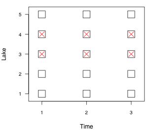
Fig. 1 A lake monitoring study with
time nested in lakes
In sampling theory a distinction is made between the population and the sample. The population is the entity P to which you want your conclusions to apply. The sample is a subset S of P. It is the set of units for which you have data.
Statistical analysis is only appropriate when we have a probability sample. A probability sample is one in which each element of the population has a known probability of being included in the sample. Typically we start with a list of all the elements in the population. This list is called the sampling frame. In a simple random sample (SRS) each element in the sampling frame has an equal probability of being included in the sample. It is a specific kind of probability sample.
A general probability sample can differ from a simple random sample in two important ways.
Simple random sampling is sometimes called unrestricted random sampling. All other samples are referred to as restricted random samples. Deviations from simple random sampling are often unavoidable.
Fig. 2 Sampling from two populations
In the frequentist approach to statistics all focus is on the sample. Suppose we draw a sample from population 1 and calculate the sample mean ![]() which we take as an estimate of the population mean μ1.
which we take as an estimate of the population mean μ1.
Similarly suppose we draw a sample from population 2 and calculate the sample mean ![]() which we take as an estimate of the population mean μ2. We observe for our two samples that
which we take as an estimate of the population mean μ2. We observe for our two samples that ![]() . Are we therefore justified in concluding that
. Are we therefore justified in concluding that ![]() ?
?
Because we only have the sample at hand on which to base our conclusions, we should hesitate in making this logical leap. If we were to go back and obtain a second sample from each population we would not expect to obtain exactly the same sample means again. Even the direction of the inequality might change the second time around. The way to address this is to quantify the expected variability of means of samples drawn repeatedly from a population. If we knew how much sample means are likely to vary in repeated sampling we can then assess whether it is likely that the order of the inequality might change in a subsequent sample.
The point of this is to just to remind you that sample means are random variables. As such, they have a distribution, called a sampling distribution. In the frequentist perspective, the precision of a sample estimate depends not on the one sample you have but on all the possible samples you might have obtained. When you engage in restricted random sampling the distribution of possible samples you might obtain is different from what it would is for unrestricted random sampling. As a result the estimate of the precision of the sample estimate changes under these different sampling regimes. Thus we need to account for the sampling design in order to draw correct inferences from samples.
In elementary statistics you learned that the variance of the sample mean is given by  and is estimated by
 ![]() . Here σ2 is the population variance, s2 is the variance of the sample, and n is the sample size.
This is a very cool formula. It tells us that in order to understand how the sample mean varies under repeated sampling we need only look at quantities that we can measure from a single sample. Coupling this result with the central limit theorem allows us to make probabilistic statements about whether μ1 is likely to be greater than μ2.
. Here σ2 is the population variance, s2 is the variance of the sample, and n is the sample size.
This is a very cool formula. It tells us that in order to understand how the sample mean varies under repeated sampling we need only look at quantities that we can measure from a single sample. Coupling this result with the central limit theorem allows us to make probabilistic statements about whether μ1 is likely to be greater than μ2.
If our sample sizes are large (or they're small but the underlying populations we're sampling from are normally distributed with known variances), then a confidence interval can be constructed for the mean difference ![]() using the standard normal distribution and the variances of the means. If this confidence interval does not contain zero and is strictly positive we can have some confidence in concluding that
using the standard normal distribution and the variances of the means. If this confidence interval does not contain zero and is strictly positive we can have some confidence in concluding that ![]() .
.
If our sample sizes are small and the underlying population is not normally distributed, but the variance is known, or the sample sizes are small and we use the sample variance as an estimate of the population variance of an underlying normal population, then we should use a t-distribution instead of a normal distribution to construct the confidence interval.
In truth the formula for the variance of the sample mean was derived assuming simple random sampling with replacement (SRSWR). When a sample is made with replacement then the element selected on the first draw has no influence on which element is selected on the second draw. The probabilities do not change. If our sample size is n and the population size is N, then the probability of drawing any single element is ![]() and the probability of drawing any two elements in succession is
and the probability of drawing any two elements in succession is ![]() .
.
Typically though we don't sample with replacement. Because populations are finite the probabilities change on each draw as the pool of available elements changes. When sampling without replacement the probability of drawing any two elements in succession is ![]() , accounting for order. When we sample without replacement from a finite population a correlation is induced between the elements in our sample and this in turn requires a modification of the formula for the variance of the sample mean.
, accounting for order. When we sample without replacement from a finite population a correlation is induced between the elements in our sample and this in turn requires a modification of the formula for the variance of the sample mean.
For a simple random sample without replacement (SRSWOR), the variance of the sample mean is given by
and is estimated with
The additional factor that appears in each of these expressions is called the finite population correction factor (FPC). Since we're usually dealing with a sample estimate we'll generally use FPC to refer to the second usage.
The ratio of the sample size to the population size that appears in the last expression is called the sampling fraction and is usually denoted by ![]() .
.
Observe that if N, the population size, is very large, then the FPC is approximately equal to 1 and can be ignored. Consequently one can think of sampling with replacement as being roughly equivalent to sampling from an infinite or, more realistically, from a very large population. In words, the FPC tells us how much extra precision we have achieved when the sample size comes close to the population size. It is to our advantage to include the FPC in our calculations because its presence decreases the variance of our estimates (making them appear to be more precise).
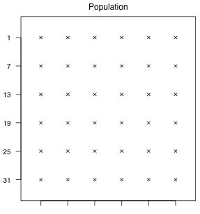
Fig. 3 is a schematic diagram of a population consisting of 36 units. We'll use this population to illustrate various sampling schemes. If it helps you can think of the diagram as representing the spatial locations of individuals in a population. The numbers on the left margin will be used to identify the individual elements in the population. We start numbering the elements from 1 in the top left corner to 36 in the bottom right corner. These numbers comprise the sampling frame for the population.
In all of our examples we will draw a sample of size 12 from this population. Thus in terms of the notation developed previously:
 |
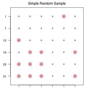 |
Fig. 3 The population of potential sample units |
Fig. 4 A simple random sample of size 12 |
There are a total of  possible simple random samples of size 12 that can be drawn from this population.
choose(36,12)
[1] 1251677700
To produce one of these samples in R we can use the sample function. The sample function has two required arguments and a third optional argument. (There is a fourth optional argument that is of no interest to us at the moment.) In default order the arguments are the following.
By default the sample function uses the internal clock value to initialize the random number stream that it uses to obtain a random sample from x. The initialization can be manually set with the set.seed function.
To obtain a random sample without replacement of size 12 from the numbers 1 through 36, use the following command.
sample(1:36, 12, replace=FALSE)
Fig. 4 illustrates the sample that was obtained.
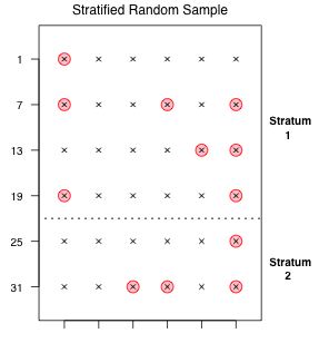
Fig. 5 A stratified random sample using
proportional allocation
The first example of a restricted random sample that we will consider is a stratified random sample. In a stratified random sample the population is assumed to consist of multiple subpopulations, called strata, and we take random samples separately from each. Assume for our schematic population that elements 1–24 make up stratum 1 and elements 25–36 make up stratum 2. We will take our random sample of size 12 in a way that guarantees that a portion of the sample comes from each stratum.
There are a number of methods for deciding how many elements to select from the different strata.
In truth any allocation scheme is OK if it can be objectively justified and the selection schemes are recorded.
I illustrate proportional allocation using our schematic population. Since the strata are in the proportions two thirds (stratum 1) to one third (stratum 2) in the population, our sample of size 12 should exhibit the same proportions. Thus we should choose 8 elements from stratum 1 and 4 elements from stratum 2. There are  different proportional allocation samples that can be drawn from this population.
choose(24,8)*choose(12,4)
[1] 364058145
We can obtain a list of elements for our stratified sample by using the R sample function twice.
One such stratified random sample is shown in Fig. 5.
| Jack Weiss Phone: (919) 962-5930 E-Mail: jack_weiss@unc.edu Address: Curriculum for the Environment and Ecology, Box 3275, University of North Carolina, Chapel Hill, 27599 Copyright © 2012 Last Revised--April 27, 2012 URL: https://sakai.unc.edu/access/content/group/2842013b-58f5-4453-aa8d-3e01bacbfc3d/public/Ecol562_Spring2012/docs/lectures/lecture41.htm |