The data are from Zuur et al. (2007) who use it to introduce classification and regression trees in their Chapter 9. The data set used to illustrate regression trees is a Bahamas fisheries data set consisting of unpublished data from The Bahamas National Trust / Greenforce Andros Island Marine Study. Zuur et al. (2007) describe the data as follows (p. 147):
Parrotfish densities are used as the response variable, with the explanatory variables: algae and coral cover, location, time (month), and fish survey method (method 1: point counts, method 2: transects). There were 402 observations measured at 10 sites.
They choose not to use CoralRichness in the analysis and we will follow suit. Because the response variable Parrot is parrotfish density, a continuous variable, we will use these data to construct a regression tree.
Zuur et al. (2007) use a second data set to illustrate classification trees. They describe the data and their objectives as follows (p. 152–153).
These data are from an annual ditch monitoring programme at a waste management and soil recycling facility in the UK. The soil recycling facility has been storing and blending soils on this site for over many years, but it has become more intensive during the last 8 to 10. Soils are bought into the stockpile area from a range of different sites locations, for example from derelict building sites, and are often saturated when they arrive. They are transferred from the stockpile area to nearby fields and spread out in layers approximately 300 mm deep. As the soils dry, stones are removed, and they are fertilised with farm manure and seeded with agricultural grasses. These processes recreate the original soil structure, and after about 18 months, the soil is stripped and stockpiled before being taken off-site to be sold as topsoil.
The main objective of the monitoring was to maintain a long-term surveillance of the surrounding ditch water quality and identify any changes in water quality that may be associated with the works and require remedial action. The ecological interest of the site relates mainly to the ditches: in particular the large diversity of aquatic invertebrates and plants, several of which are either nationally rare or scarce. Water quality data were collected four times a year in Spring, Summer, Autumn and Winter, and was analysed for the following parameters: pH, electrical conductivity (μS/cm), biochemical oxygen demand (mgl–1), ammoniacal nitrogen (mgl–1), total oxidised nitrogen, nitrate, nitrite (mgl–1), total suspended solids (mgl–1), chloride (mgl–1), sulphate (mgl–1), total calcium (mgl–1), total zinc (μgl–1), total cadmium (μgl–1), dissolved lead (μgl–1), dissolved nickel (μgl–1), orthophosphate (mgl1) and total petroleum hydrocarbons (μgl–1). In addition to water quality observations, ditch depth was measured during every visit. The data analysed here was collected from five sampling stations between 1997 and 2001. Vegetation and invertebrate data were also collected, but not used in this example.
The underlying question now is whether we can make a distinction between observations from different ditches based on the measured variables.
The response variable, Site, is a categorical variable with five categories and hence will be used to construct a classification tree.
The Ditch data set contains only 48 observations. This makes it less than ideal for building a tree model.
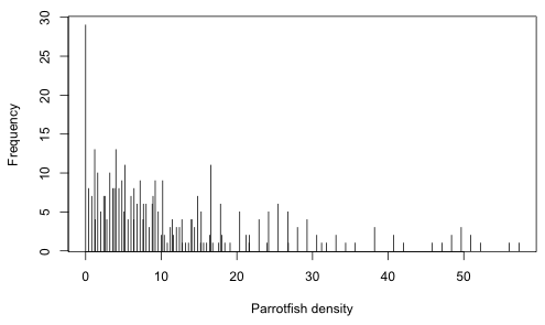
It's worth considering how we might analyze the Bahama data using a parametric regression model. Regression trees are indifferent to nature of the response variable but this does matter when choosing a probability distribution for a parametric model. The variable of interest, parrotfish density, presumably was obtained by counting parrotfish and dividing the total by the area surveyed. While this may seem like a perfectly natural variable, ratios can be exceedingly difficult to analyze statistically. We can get a sense of the difficulty when we look at the distribution of the parrotfish density variable (Fig. 1).
|
| Fig. 1 Distribution of parrotfish densities |
Fig. 1 is a bar chart of the different parrotfish densities in the data set. Keep in mind that the overall distribution of the response is largely irrelevant in regression. Instead it is the distribution of the response at various predictor combinations that matters. Because density is a non-negative quantity and we see from the graph that much of the data is close to and even achieves its lower boundary of zero, a distribution that permits negative values such as a normal distribution is not likely to be a good choice here. If we turn to positive distributions such as the lognormal and gamma we find there is another problem. These distributions don't allow zero values.
Yet 7% (n = 29) of the observed parrotfish densities are zero. One solution is to assume the zeros aren't really zero, but are small positive numbers that fall below our detection threshold. Alternatively we could analyze the zeros separately by fitting a binomial model to the presence-absence of parrotfish. Then conditional on parrotfish being present we could fit a lognormal model to the nonzero densities. Splitting up the data like this diminishes our ability to detect effects of interest. It is quite likely that the factors that cause density to be low also cause density to be zero.
All of these issues have arisen because we've chosen to record the response variable as density. The actual variable in nature is a count, the number of parrotfish observed on a transect, which we then chose to divide by the area surveyed. If the transects vary in length then the number of fish observed will vary also, so we need to control for area. Rather than forming a ratio we can control for the effect of area by including it in the regression model as a covariate.
The advantage of doing it this way is that the response variable is still a count and we can make use of probability models for counts (Poisson, negative binomial, etc.) all of which permit a count to be equal to zero.
If we insist that the results be interpretable as effects on density then there is yet another option: use parrotfish counts as the response variable but use log(area) as an offset rather than as a predictor. An offset is a term in a regression model whose coefficient is constrained to be 1. In R we would fit a model with an offset as follows.
Because the default link function for Poisson regression is a log link, the above syntax fits the following regression model.
where the last step follows from a property of logarithms. So if we assume parrotfish counts have a Poisson distribution (which allows zeros), then by including log area as an offset we end up with a model for density. The same result holds if the parrotfish counts are assumed to have a negative binomial distribution. The bottom line is that fitting models to densities is a messy statistical problem, while fitting models to counts is easy. Avoid working with densities unless you have no other choice.
Regression trees are fit with the rpart function in the the rpart package. The default syntax is identical to that which we've used with most of the regression functions of R. Because Month, Station, and Method are recorded with numerical values I declare them as factors explicitly in the model formula. Because Parrot is a continuous variable, rpart fits a regression tree. To explicitly request a regression tree we can add the argument method="anova".
The default print method for rpart is to print a text representation of the tree. Generally you shouldn't use the summary function on an rpart object unless you want to see all the details of the tree construction.
node), split, n, deviance, yval
* denotes terminal node
1) root 402 50190.0 10.780
2) as.factor(Method)=2 244 7044.0 6.449
4) CoralTotal< 4.955 87 1401.0 3.526 *
5) CoralTotal>=4.955 157 4488.0 8.069
10) as.factor(Station)=2,3,6,7,10 122 2593.0 7.075 *
11) as.factor(Station)=1,5,9 35 1355.0 11.530 *
3) as.factor(Method)=1 158 31490.0 17.470
6) as.factor(Station)=3,4 25 781.7 3.157 *
7) as.factor(Station)=1,2,5,6,7,8,9,10 133 24630.0 20.160
14) as.factor(Month)=5,7,8,10 94 11590.0 17.090
28) as.factor(Station)=1,5,6,7,8 66 6717.0 15.530 *
29) as.factor(Station)=2,9,10 28 4328.0 20.780 *
15) as.factor(Month)=11 39 10020.0 27.560
30) CoralTotal>=4.395 27 7647.0 24.810 *
31) CoralTotal< 4.395 12 1713.0 33.740 *
Each line of the text tree contains the following information.
Each split leads to a reduction in total deviance. At the root (null) node the total deviance is 50,190.0. After the first split the total deviance is reported to be
so the deviance has been reduced by splitting on the variable Method. At each stage of the tree we can sum the deviances at all the terminal nodes and compare it to the deviance at the root node to obtain an R2, the fraction of the original total deviance that has been explained by the tree.
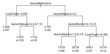
Thus splitting the data set into groups based on the variable Method and using the mean response in each group as the predicted value has explained 23% of the original variability in parrotfish density. We can obtain a graphical summary of the regression tree by plotting the rpart object and then using the text function to add labels to the nodes.
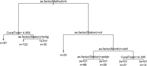 |
| Fig. 2 Graphical display of the tree |
The margin= argument in plot expands the white space around the tree to prevent truncation of the text that comes next. The use.n= argument of text adds the information about the number of observations occurring at each of the terminal nodes. Notice that rpart has relabeled the categories of each factor variable as a, b, c, etc. This is to avoid overlap with long category names. We can get the actual category levels to display by including the pretty argument of text. Setting pretty=1 causes the numeric category levels to be printed.
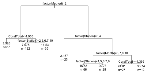 |
| Fig. 3 Tree with argument pretty=1 |
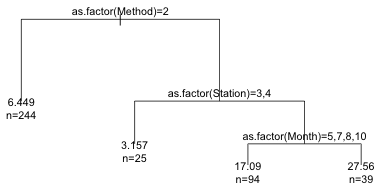
By default the tree is drawn so that the length of the branches indicate the relative magnitudes of the drops in deviance at each split point. This typically means that the information in the terminal leaves gets crowded together because the changes in deviance there are relatively small. We can correct this by adding the uniform=T argument to plot to obtain trees with equal branches.
 |
| Fig. 4 Tree with uniform branching |
We can change the appearance of the branches with the branch argument. The default choice is branch=1 which yields the rectangular shoulders shown. Choosing branch=0 yields branches with no shoulders. Intermediate values for branch yield trees with shorter shoulders. I leave out the pretty argument to obtain a more compact display.
(a)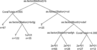 |
(b)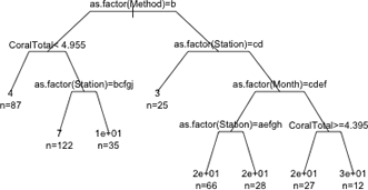 |
Fig. 5 The effect of varying the branch argument on the displayed tree. (a) branch=0; (b) branch=0.5. Figs. 2, 3, and 4 show branch=1. |
|
We can obtain the value of the cost complexity parameter for trees of different sizes with the printcp function.
Variables actually used in tree construction:
[1] as.factor(Method) as.factor(Month) as.factor(Station) CoralTotal
Root node error: 50188/402 = 125
n= 402
CP nsplit rel error xerror xstd
1 0.232 0 1.00 1.00 0.116
2 0.121 1 0.77 0.77 0.083
3 0.060 2 0.65 0.71 0.075
4 0.023 3 0.59 0.67 0.071
5 0.013 4 0.56 0.64 0.072
6 0.011 5 0.55 0.65 0.073
7 0.011 6 0.54 0.64 0.071
8 0.010 7 0.53 0.63 0.069
While relative error is guaranteed to decrease as the tree gets more complex, this will not normally be the case for cross-validation error. Because the cross-validation error is still decreasing in the output shown above, the default tree size is probably too small. We need to refit the model and force rpart to carry out additional splits. This can be accomplished with the control argument of rpart. I use the rpart.control function to specify a value for cp= that is smaller than the default value of 0.01. Because the cross-validation error results are random, I use the set.seed function first to set the seed for the random number stream so that the results obtained are reproducible.
The CP table exists as a component of the rpart object.
From the output it appears that xerror has achieved an interior minimum. We can obtain an informative graphical display of the cp table with the plotcp function.
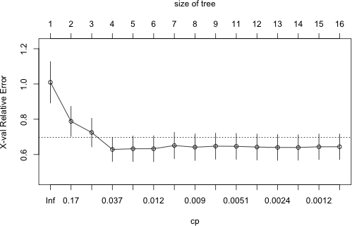 |
Fig. 6 Plot of CP table. The dotted line denotes the upper limit of the one standard deviation rule. |
From the graph it would appear that the minimum cross-validation error occurred for the fourth tree listed in the CP table that had a total of 4 leaves. We can verify this by just examining the table by eye or more formally as follows.
So, if we were to use the tree that minimized the cross-validation error we would choose a tree with 3 splits. As was noted in lecture 36, the problem with such a choice is that the cross-validation error is a random quantity. There is no guarantee that if we were to fit the sequence of trees again using a different random seed that the same tree would minimize the cross-validation error.
A more robust alternative to minimum cross-validation error is to use the one standard deviation rule: choose the smallest tree whose cross-validation error is within one standard error of the minimum. Using this rule we would still end up with the same tree. The first tree whose point estimate of the cross-validation error falls within the ± 1 xstd of the minimum, is the minimum tree itself of size 4. I extract the CP value of this tree and refit the tree using the prune function on the current tree object.
node), split, n, deviance, yval
* denotes terminal node
1) root 402 50190.0 10.780
2) as.factor(Method)=2 244 7044.0 6.449 *
3) as.factor(Method)=1 158 31490.0 17.470
6) as.factor(Station)=3,4 25 781.7 3.157 *
7) as.factor(Station)=1,2,5,6,7,8,9,10 133 24630.0 20.160
14) as.factor(Month)=5,7,8,10 94 11590.0 17.090 *
15) as.factor(Month)=11 39 10020.0 27.560 *
 |
| Fig. 7 The pruned tree |
This result is probably the researcher's worst nightmare. None of the important predictors turn out to be biological variables. Instead we see that the survey method (point counts versus transect) is the most important predictor of parrotfish density. The right branch consisting of only point counts then divides out best by the location at which the sample was taken (station) and six of these stations are then split by the month of the sample.
The predict function works with tree objects. For a regression tree it returns the mean at the leaf where the observation is assigned.
Just like the rpart object, the prune object contains quite a bit of information.
The $where component indicates to which leaf the different observations have been assigned.
The numbers themselves correspond to row numbers in the $frame component that defines the final tree.
Notice that rows 2, 4, 6, and 7 are labeled as leaves but have row names 2, 6, 14, and 15. The row names in the frame are the actual left-to-right positions of the leaves in the tree. The missing numbers correspond to splits and leaf locations that don't appear in the pruned tree. We can use all this information to display box plots in the same order as the left-to-right positions of the leaves of the pruned tree. I adjust the margins of each graph with the mar argument of par to try to position the boxplots right below the corresponding leaf of the tree. I use the contents of the $where component to group the observations by their final leaf assignment.
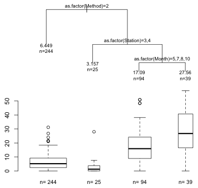 |
Fig. 8 Pruned tree with box plots of the distributions of the response at the terminal nodes |
Based on the box plots it appears that the first two splits of the tree have managed to pull out most of surveys that yielded the lowest densities of parrotfish.
The partykit package of R produces enhanced displays of regression and classification trees. It does its own version of Fig. 8. To use it we need to convert the tree created by rpart into a party object with the as.party function. I pass an additional argument, id=FALSE, to the plot function to suppress displaying the node number of each tree.
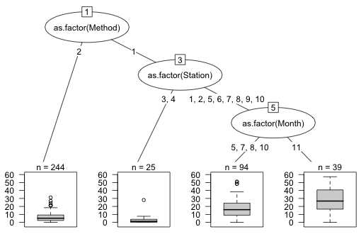 |
Fig. 9 Regression tree diagram produced by the partykit package |
Classification trees are constructed the same way as regression trees, so I skip over most of the preliminaries. The data in the Ditch data set are clearly heterogeneous but perhaps we can ignore this because we're treating the annual measurements at each site as replicates of that site. I start with a small value for cp so that the initial tree is as large as possible. Because we don't have much data (only 48 observations) I also set a lower value for the minsplit criterion. By default it's set at 20 so that any group with fewer than 20 observations in it would not be split further. (Note: by default minbucket, the minimum number of observations allowed to form a terminal node, is set to minbucket = minsplit/3 so reducing minsplit also decreases minbucket.) The default split criterion is the Gini index. This can be changed to the entropy measure. To carry this out we would need to add a parms argument to the rpart call: parms=list(split="information").
To avoid typing all of the variable names in the model formula I use the ~. notation and remove those variables that should not be in the model by not including them in the data argument. To obtain a classification tree the response variable needs to be a factor. Alternatively one can add the argument method='class' to obtain a classification tree.
node), split, n, loss, yval, (yprob)
* denotes terminal node
1) root 48 38 1 (0.21 0.19 0.21 0.21 0.19)
2) Total_Calcium>=118 25 16 5 (0.32 0.28 0 0.04 0.36)
4) Conductivity< 1505 11 6 1 (0.45 0.45 0 0.091 0) *
5) Conductivity>=1505 14 5 5 (0.21 0.14 0 0 0.64) *
3) Total_Calcium< 118 23 13 3 (0.087 0.087 0.43 0.39 0)
6) Depth>=0.505 8 0 3 (0 0 1 0 0) *
7) Depth< 0.505 15 6 4 (0.13 0.13 0.13 0.6 0)
14) Conductivity< 622.5 5 3 1 (0.4 0 0.4 0.2 0) *
15) Conductivity>=622.5 10 2 4 (0 0.2 0 0.8 0) *
The output resembles that of the regression tree with the following differences.
I next display a graph of the tree.
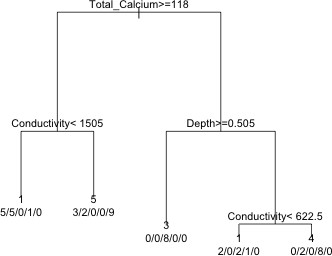 |
| Fig. 10 A classification tree |
At each leaf we have the predicted category for the members of that leaf using a simple majority rule. The use.n=T argument caused the actual number of observations in the five categories to be displayed below the prediction.
I next generate a plot of the cross-validation error for different values of cost complexity parameter.
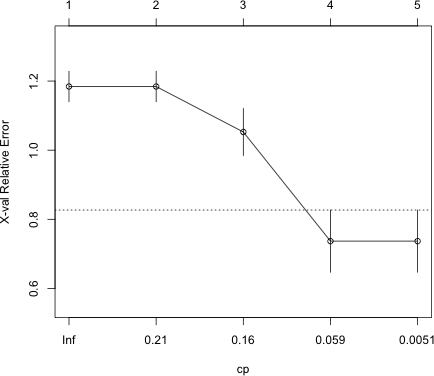 |
Fig. 11 The cross-validation error for a sequence of classification trees |
The result are fairly unambiguous. A tree with four leaves is best. I examine the CP table.
I prune the tree using the optimal value of CP and display the results.
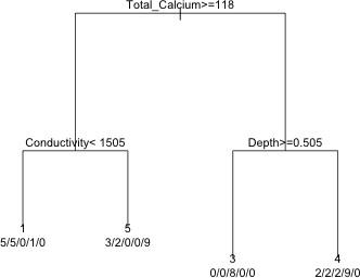 |
| Fig. 12 The pruned tree |
The predict function applied to classification trees reports the category probabiities for the leaf that an observation is assigned.
The default partykit display for classification trees is a bar chart for response variables with more than two categories. Based on the displayed frequency counts in the leaves it's clear that we've classified one group perfectly and two others fairly well.
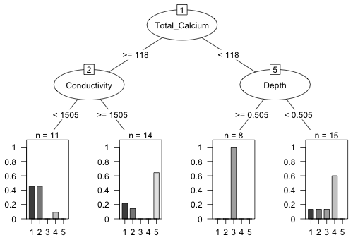 |
Fig. 13 Classification tree diagram produced by the partykit package |
Another way we can summarize the classification results graphically is with a mosaic plot, which replaces the box plots for a regression tree and the bar charts produced by the partykit package.
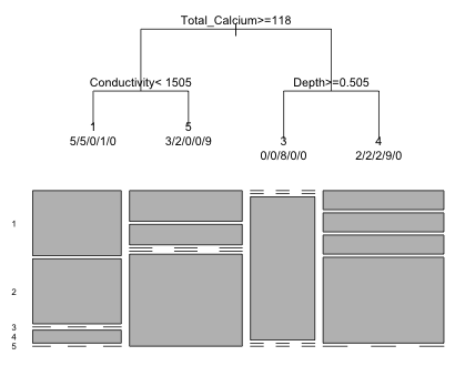 |
Fig. 14 Classification tree and corresponding mosaic plot |
In a mosaic plot the categories that don't appear at a leaf are shown with dashed lines in the appropriate positions. The width of the boxes reflect the number of observations assigned to the four leaves of the tree.
The first split of the classification tree was based on calcium levels. We can graphically assess how well this split discriminated the sites with a dot chart in which a line is superimposed at the calcium split value. Each site type is displayed with a different symbol type.
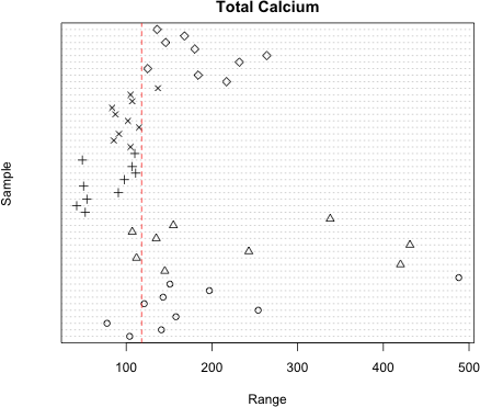 |
Fig. 15 Dot plot of the primary split variable, Total_Calcium |
From the graph it's pretty clear that total calcium level does a very good job at discriminating two groups of sites. Sites 1, 2, and 5 look very different from sites 3 and 4. For most of the sites only a couple of years end up being classified into the wrong group, while site 3 has been classified perfectly.
So far we've been ignoring the summary results from an rpart run because the output is so copious. It contains an entire summary of the tree fitting process. One useful portion of the summary output is the description of surrogate splits. Below I show this information for the first split at Total_Calcium.
CP nsplit rel error xerror xstd
1 0.23684 0 1.0000 1.1842 0.04413
2 0.18421 1 0.7632 1.1842 0.04413
3 0.13158 2 0.5789 1.0526 0.06795
4 0.02632 3 0.4474 0.7368 0.08989
Node number 1: 48 observations, complexity param=0.2368
predicted class=1 expected loss=0.7917
class counts: 10 9 10 10 9
probabilities: 0.208 0.188 0.208 0.208 0.188
left son=2 (25 obs) right son=3 (23 obs)
Primary splits:
Total_Calcium < 118 to the right, improve=6.392, (0 missing)
Chloride < 71 to the right, improve=6.142, (0 missing)
Sulphate < 205 to the right, improve=5.792, (0 missing)
Conductivity < 703 to the right, improve=5.125, (0 missing)
Depth < 0.505 to the right, improve=4.807, (4 missing)
Surrogate splits:
Chloride < 71 to the right, agree=0.917, adj=0.826, (0 split)
Conductivity < 722.5 to the right, agree=0.896, adj=0.783, (0 split)
Sulphate < 261 to the right, agree=0.875, adj=0.739, (0 split)
Ammoniacal_Nitrogen < 0.25 to the right, agree=0.812, adj=0.609, (0 split)
Total_Zinc < 0.035 to the right, agree=0.708, adj=0.391, (0 split)
The section labeled "Primary splits" lists the top five options that were considered for forming the first split. From this we can see that Total_Calcium was not a clear winner. Chloride, the second choice, does nearly as well in decreasing impurity. If the goal in building a classification tree is to screen out variables for a subsequent parametric regression, then one might consider including some of competitive primary split variables in the parametric regression too.
The section labeled Surrogate splits considers other splits that most closely agree with the group allocations obtained with Total_Calcium < 118. For instance we see that choosing to split on Chloride < 71 instead of Total_Calcium < 118 would have yielded a classification of observations at this split that is 91.7% in agreement. This can be useful in predicting new observations that have missing values for the primary split variable. So if a new variable did not have a value for Total_Calcium we could use Chloride instead and most likely achieve a similar classification to what we would have if we had a value for Total_Calcium.
Two R packages that implement random forests are randomForest and party. The randomForest package is an R port of the Fortran code of the original implementation of random forests by Leo Breiman. The party package uses conditional inference trees that supposedly minimize the bias that random forests can exhibit with correlated variables. The function in the randomForest package for fitting random forests is randomForest. It uses a formula interface just like rpart.
Unlike rpart we need to tell the randomForest function how to deal with missing values because randomForest needs to construct subsets of the variables when building individual trees. A standard choice is na.action=na.roughfix. This imputes missing values using either the median of the non-missing observations (regression trees) or the most frequent category (classification trees). I add this argument as well as importance = T in order to obtain importance statistics.
If we print the object we get details about the fit.
OOB estimate of error rate: 47.92%
Confusion matrix:
1 2 3 4 5 class.error
1 1 4 2 0 3 0.9000000
2 5 3 0 0 1 0.6666667
3 0 0 7 2 1 0.3000000
4 1 0 2 7 0 0.3000000
5 1 0 0 1 7 0.2222222
From the printout we see that by default the forest was built from 500 trees each of which is a bootstrap sample from the actual data. Observations that are left out of the bootstrap sample form the "out of bag" (OOB) set. The OOB observations from each tree were used to assess fit. The printout reports that at each split point a random sample of three predictors (= the floor of the square root of the total number of predictors) was obtained and used to determine the best split.
The error rate of 47.92% can be calculated from the confusion matrix shown at the bottom of the output. The rows of the confusion matrix correspond to the actual categories while the columns are the predicted categories. The predictions of the OOB observations are based on the majority opinion of the 500 trees. Entries on the diagonal are the number of times the random forest made the correct prediction. Thus we see that in site 1 only one of the observations was correctly predicted by the forest; the other nine were incorrectly assigned to other categories. The best prediction rate is for site 5 where 7 of the 9 observations are correctly classified by the random forest.
By specifying importance=T in the function call we obtain measures of each variable's importance to the classification.
The two columns labeled MeanDecreaseAccuracy and MeanDecreaseGini contain the two importance measures discussed in lecture 36. MeanDecreaseAccuracy measures how much the prediction is affected if the values of a predictor are randomly permuted among the other observations in the OOB set. A good way to display these results is with a dot chart in which the variables are sorted by their importance.
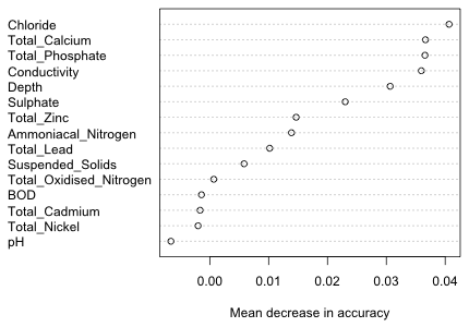 |
Fig. 16 Variable importance as indicated by the mean decrease in accuracy |
The variables appear to fall roughly into groups with the first five or six variables being clearly more important than the rest. It's useful to compare this picture to the one we get using the importance measure based on the Gini index.
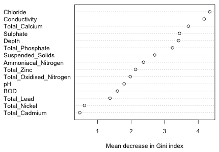 |
Fig. 17 Variable importance as determined by the mean decrease in Gini index |
While there has been a change in the order of the variables, the first six ranked variables using either importance measure are the same.
The predict function works with randomForest objects. By default, the predict function returns the majority vote of the 500 trees for the times when that the observation was OOB.
If type='prob' is added as an argument we get instead the proportion of times that a given observation was assigned to the different categories while OOB.
Zuur, Alain F., Elena N. Ieno, and Graham M. Smith. 2007. Analysing Ecological Data. Springer, New York. UNC e-book
| Jack Weiss Phone: (919) 962-5930 E-Mail: jack_weiss@unc.edu Address: Curriculum for the Environment and Ecology, Box 3275, University of North Carolina, Chapel Hill, 27599 Copyright © 2012 Last Revised--April 17, 2012 URL: https://sakai.unc.edu/access/content/group/2842013b-58f5-4453-aa8d-3e01bacbfc3d/public/Ecol562_Spring2012/docs/lectures/lecture37.htm |