Lecture 35—Monday, April 9, 2012

Outline of lecture

• Model-based and algorithm-based approaches to statistics
• Binary recursive partitioning—heuristic description
• The recursive partitioning algorithm—formal description
• References
• R code used to produce figures

Model-based and algorithm-based approaches to statistics

So far in this course we've focused exclusively on what is called a model-based approach to statistics. In statistics a model is a proposal for how we think our data could have been generated. A statistical model contains both a systematic and a random component each of which has to specified by us. Model-based approaches while intuitively appealing have some obvious problems associated with them.

1. Somehow we have to come up with the model. While the choice of random component may be more or less obvious given the nature of the data, we still need to decide which variables to use to describe the systematic portion of the model.
2. Variable selection itself is very model-specific.
   1. If we use linear regression, then we will end up selecting only those variables that have an additive and a linear relationship to the response.
   2. If we start with a log-transformed response and use linear regression, then we will select those variables that have an additive and a linear relationship to the response on a log scale. On the original scale, these same variables will necessarily have a multiplicative effect on the response.
3. Nonlinear relationships complicate things further as the number of possible functional forms to investigate is endless. These range from truly nonlinear models to nominally nonlinear models, such as polynomial models, that can still be fit as ordinary regression models. If we use a generalized additive model (GAM) then we can address the general problem of nonlinearity without worrying about the specific functional form, but we are still forced to assume that the different variables have an additive effect on the response.
4. All of this ignores the possibility that the variables affect the response interactively. The presence of interactions complicates model formulation by an order of magnitude.

There is another approach to statistical modeling in which the actual model itself is secondary. Instead the algorithm used to obtain the model takes center stage. In a regression setting, this algorithm-based approach is generally some variation of what's called recursive binary partitioning (implemented in the rpart package of R). It is also called CART, an acronym for classification and regression trees, but this is also the name of a commercial product developed by one of the pioneers in this area, Leo Breiman (Breiman et al. 1984).

Binary recursive partitioning is typically lumped into a category of methods that are referred to as "machine learning" or "statistical learning" methods. Members of this group include support vector machines, neural networks, and many others. These methods have virtually nothing in common with each other except for the fact that they originated in the field of computer science rather than statistics. In some cases computer scientists reinvented methodologies that already had a long history in statistics. In doing so they managed to create their own terminology leaving us today with different descriptions of otherwise identical methods. As a result much of modern statistical learning theory is an awkward amalgamation of computer science and statistics. Good introductions to this area include Berk (2008) and Hastie et al. (2009). Introductory treatments for ecologists are Fielding (1999) and Olden et al. (2008).

Binary recursive partitioning—heuristic description

In binary recursive partitioning the goal is to partition the predictor space into boxes and then assign a numerical value to each box based on the values of the response variable for the observations assigned to that box. At each step of the partitioning process we are required to choose a specific variable and a split point for that variable that we then use to divide all or a portion of the data set into two groups. This is done by selecting a group to divide and then examining all possible variables and all possible split points of those variables. Having selected the combination of group, variable, and split point that yields the greatest improvement in the fit criterion we are using, we then divide that group into two parts. This process then repeats.

For a continuous response the object that is created is called a regression tree, whereas if the response is a categorical variable it's called a classification tree. Classification and regression trees are collectively referred to as decision trees. The usual fit criterion for a regression tree is the residual sum of squares, RSS. The construction of a generic regression tree model would proceed as follows.

1. Initially the RSS is the sum of squared deviations of the individual values of the response variable about their overall mean. This is called the null (root) RSS.
2. Next examine each variable and each possible split point for dividing the data into two regions. For each choice calculate the mean of the response variable and the residual sum of squares in each region separately. Sum them to obtain the total residual sum of squares for this partition and compare it to the null RSS. Identify the variable and split point that yields the greatest reduction in the RSS from the null model.
3. For all the individual regions created so far, examine each variable and possible split point again to see if one of the current regions can be divided further. For each new division calculate the mean of the response variable and the new RSS. Sum the RSS from all regions, new and old, to obtain the RSS for this partition. Compare it to the previous RSS and choose the variable, split point, and region that yields the greatest reduction in the RSS.
4. Repeat step 3 until the stopping criterion is met.

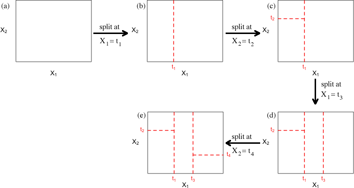
Fig. 1 illustrates a toy example of this process with only two variables X₁ and X₂. The rectangle shown in each panel is meant to delimit the range of the two variables. Here's a possible scenario for how the regression tree might evolve.

1. At the first step using the RSS criterion we choose to split the X₁ axis into two parts at X₁ = t₁ yielding Fig. 1b.
2. We next examine the two rectangles just created in turn and find that the next best split is obtained using X₂ = t₂ . This splits the left hand rectangle into two parts, Fig. 1c.
3. We now have three rectangles to examine and we find that splitting the right hand rectangle at X₁ = t₃ yields the optimal split, Fig. 1d.
4. Of the four rectangles remaining we find that the optimal next split is of the right hand rectangle using X₂ = t₄ yielding the five rectangles shown in Fig. 1e.
5. At this point our stopping criterion is met and the algorithm terminates.

Fig. 1  Heuristic example of binary recursive partitioning with a predictor set consisting of two variables X₁ and X₂

This yields the five rectangular regions R₁, R₂, R₃, R₄, and R₅ shown in Fig. 1e and Fig. 2a. Next we summarize the response variable by its mean, , , , , and , in each region. In an ordinary regression model with two variables, the regression model is visualized as a surface lying over the X₁-X₂ plane. For a model linear in X₁ and X₂, the surface is a plane. If the model contains a cross-product term X₁X₂, then the surface is curved. The model underlying a binary recursive partition can be visualized as a step surface such as the one shown in Fig. 2b. Over each of the regions shown in Fig. 2a we obtain a rectangular box whose cross-section is the given rectangular region and whose height is the mean of the response variable in that region.

(a)	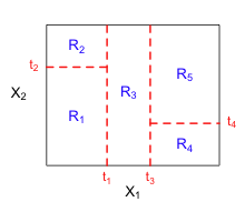(b)
Fig. 2 (a) The rectangular regions in the X1-X2 plane that were defined by the binary recursive partition shown in Fig. 1. (b) The regression surface for the response that corresponds to this binary recursive partition. Each box in (b) lies on one of the rectangular regions in (a) and its height corresponds to the mean of the response variable over that region.

The formula for the regression surface in Fig. 2b is the following.

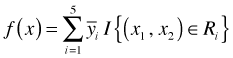
Here I is an indicator function that indicates whether the observation lies in the given rectangular region. Because an observation can only occur in one of the five regions, four of the terms in this sum are necessarily zero for each observation. As a result we just get for the region that contains the point.

Because at each stage of the recursive partition we are only allowed to divide previously split single regions, the algorithm itself can be visualized as a tree. Fig. 3a shows the tree that corresponds to the regions defined in Fig. 2a. The splitting rules used at the various steps of the algorithm are given at the branch points. By following the branches of the tree as dictated by splitting rules we arrive at the rectangular regions shown in Fig. 2a.

(a)	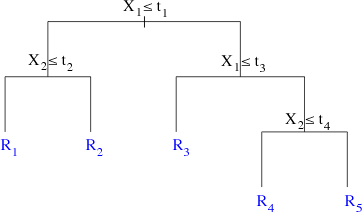(b)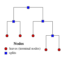
Fig. 3  (a) When we focus on the algorithm itself binary recursive partitioning yields a binary tree. (b) The terminology associated with regression and classification trees

The branching points are called splits and branch endpoints are called leaves (or terminal nodes). Both the splits and the leaves are referred to as nodes (Fig 3b). In the heuristic tree of Fig. 3b there are four splits and five leaves for a total of nine nodes.

The recursive partitioning algorithm—formal description

Step 1: Choose a variable and a split point.

For a continuous or ordinal variable with m distinct values, ξ₁, ξ₂, …, ξ_m, consider each value in turn. Each selection produces a partition consisting of two sets of values: and , i = 1, 2, … , m. Splits can only occur between consecutive data values. Thus there are m–1 possible partitions to consider. For a categorical (nominal) variable with m categories we have to consider all possible ways of assigning the categories to two groups. The splits can be anywhere and any category can be assigned to any group. Combinatorial arguments tell us that there are ways in which this can be done. (With m categories there are 2^m different subsets. Because the complement of each subset is another subset this corresponds to 2^m–1 splits. One of the subsets includes everybody (or nobody) which is not a split so we reduce this number further by 1.)

Step 2: For each possible division calculate its impurity.

Different measures of impurity are used for continuous and categorical predictors.

Continuous response: For a continuous response y, suppose we select variable X_j and split point s that yield the following two groups.

and

The usual measure of impurity used for continuous variables is the residual sum of squares. For the observations assigned to each group we calculate the mean of the response variable. The residuals sum of squares, RSS, for the current split is defined as follows.

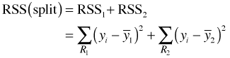
Before the data are split we calculate the overall residual sum of squares using the mean of all values of the response variable.

So for a continuous response we examine each variable X_j and all possible split points s and choose the one for which RSS₀ – RSS(split) is the largest.

Categorical response: For categorical variables there are a number of different ways of calculating impurity. Let y be a categorical variable with m categories. Let

n_ik = number of observations of type k at node i

p_ik = proportion of observations of type k at node i

The following four measures of impurity are commonly used.

1. Deviance:
2. Entropy:
3. Gini index:
4. Misclassification error: where k(i) is the category at node i with the largest number of observations.

The impurity for a given partition is the sum of the impurities over all nodes, . For a categorical variable all four measures of impurity are minimized when all the observations at a node are of the same type. The goal in a classification tree is to choose splits that yield groups that are purer than in the current partition.

Step 3: Try to partition the current groups further. Having chosen a best partition at the current stage of the tree, we next try to partition each of the groups that were formed by considering all nodes in turn. We are only allowed to partition within existing partitions (not across partitions). It is adherence to this rule that produces the tree structure.

Step 4: At some point stop. The issue of stopping rules is discussed next time.

References

• Berk, Richard A. 2008. Statistical Learning from a Regression Perspective. New York: Springer-Verlag.
• Breiman, Leo, Jerome Friedman, Richard A. Olshen, and Charles J. Stone. 1984. Classification and Regression Trees. Boca Raton, FL: Chapman & Hall.
• Fielding, Alan. 1999. Machine Learning Methods for Ecological Applications. Norwell, MA: Kluwer Academic Publishers.
• Hastie, Trevor, Robert Tibshirani, and Jerome Friedman. 2009. The Elements of Statistical Learning: Data Mining, Inference, and Prediction. New York: Springer-Verlag.
• Olden, J. D., J. J. Lawler, and N. L. Poff. 2008. Machine learning methods without tears: a primer for ecologists. Quarterly Review of Biology 83(2): 171–193.
  

R code for figures

Course Home Page