Lecture 27—Monday, March 19, 2012

Topics

• The basics of survival analysis
  • Types of censoring
  • Standard statistical methods don't work well with survival data
• The survivor and hazard functions
• The basic activities of survival analysis
• The Kaplan-Meier estimator of the survivor function

The basics of survival analysis

The subject matter of survival analysis, also called event history analysis, is the "time to an event." Events in ecology might include the following.

1. Death (in which case we're truly talking about survival).
2. Time to reproduction. Notice that in this case there is the possibility of recurrent events for polycarpic (plants) or iteroparous (animals) species.

Although the language is clearly loaded, the "time to an event" is usually called a survival time and the event itself is typically called a failure regardless of the kind of event.

For events that may or may not occur during a study period, a possible alternative to survival analysis is logistic regression. Logistic regression focuses exclusively on whether an event occurs and ignores the time profile of the events. It also fails to distinguish true negatives from false negatives. In survival analysis, on the other hand, the focus is on the time profile of events rather than the raw number of events and the problem of false negatives is dealt with explicitly.

There are two primary reasons why survival analysis requires its own methodology.

1. Survival time distributions are non-normal and are typically long-tailed. In the parametric approach to survival analysis some rather exotic probability distributions are used that are quite unlike those used in other applications.
2. Survival times are subject to censoring. A censored observation is one in which we have some information about survival time, but we don't know the survival time exactly. For example, an observation is censored if the study ends before the event has occurred. An observation may also be treated as censored if the observation "fails" because the observation dropped out of the study for a reason unrelated to the event of interest.

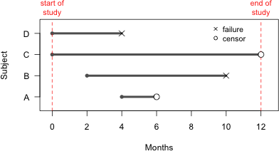
Fig. 1 illustrates the survival history for four seedlings that are part of a plant restoration study. Adults were introduced into different portions of the historical range of the species from which the species has been extirpated. To assist in returning the species to the wild the goal was to discover which habitats promote plant longevity and reproductive success.

Fig. 1  Survival histories of four re-introduced seedlings

Time lines in Fig. 1 begin at the point when the seedling was first observed in the field and end when the seedling was last observed. Individuals B and D experienced events (death) while individuals A and C were censored. Individual C was still alive when the study concluded. Individual A was stepped on by a field worker and so its death was not considered a natural death. The organization of the raw data corresponding to the graphical display of Fig. 1 is shown in Table 1.

As is often the case with survival data, the subjects exhibited a staggered entry with respect to calendar time. Survival analysis per se deals with time durations, the length of time a subject is observed. For this purpose each subject has a starting time of zero and an ending time that occurs when it experiences an event or leaves the study for other reasons. The variable Age in Table 1 records the length of time of each subject was observed to be alive while Status specifies the nature of the last observation time, 1 for an event and 0 if censored. The different symbols used at the endpoint of each time line in Fig. 1 also reflects each subject's value of Status.

Types of censoring

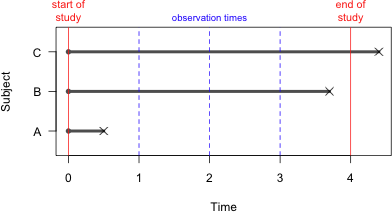
A censored individual provides some information but just not as much information as an observation that experienced an event. The amount of information it provides depends on the nature of the censoring. There are three basic kinds of censoring and these are distinguished in Fig. 2.

Fig. 2  An illustration of the different types of censoring: right censoring (subject C), left censoring (subject A), and interval censoring (subject B). Subjects are only observed at times 1, 2, 3, and 4.

1. Right censoring—the event follows the last observation time so that the observed survival time is less than the true survival time. Right censoring is the most common form of censoring because it corresponds to any observations who have not experienced the event of interest at the conclusion of the study. In our seedling example, if a given seedling is age t at the conclusion of the study then the best we can say is that the seedling's failure time is represented by the interval (t, ∞). Subject C in Fig. 2 is right censored.
2. Left censoring—the event precedes the first observation time so that the observed survival time is greater than the true survival time. As an example, suppose a seedling is known to exist at baseline but at the first official observation time, one month later, the seedling is nowhere to be found. Thus its survival time is less than t = 1 and could be represented as (0, t). This is subject A in Fig. 2.
3. Interval censoring—the event occurs between two observation times a and b so that the precise time of the event is not known. Clearly left censoring is a special case of interval censoring (as, in truth, is right censoring). Subject B in Fig. 2 is interval censored.

The objective of survival analysis is to use all the information provided by the censored individual up until the time of censoring.

Standard statistical methods don't work well with survival data

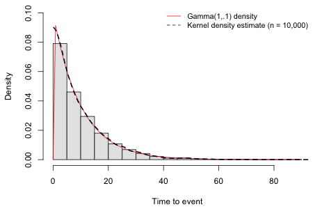
I simulate 10,000 observations from a Gamma(1, .1) density, a long-tailed probability distribution that is sometimes used as a model for survival data. The theoretical density and the density estimated from this sample of 10,000 are shown in Fig. 3. As we can see the sample estimate of the density is quite close to the theoretical curve.

Fig. 3  A gamma(1, .1) density and an empirical estimate of this density based on a random sample of size 10,000.

The theoretical mean of a Gamma(a, b) distribution is , which is equal to 10 in the example of Fig. 3. The estimate of the mean we obtain using the random sample of size 10,000 is quite close to this.

Now suppose that these data were obtained as part of an experiment that we had to terminate at time = 25 so that event times in excess of 25 are censored. This corresponds to 8.4% of the observations.

If we simply delete those observations we seriously underestimate the mean survival time.

If we instead assign the censored values their last observation time, 25, we still underestimate the mean.

It's worth noting that the median is unaffected by this kind of censoring as long as we retain the censored observations. On the other hand, if censoring occurred at various times throughout the study the median can also be affected. The primary motivation behind survival analysis is that it provides us with procedures for obtaining good estimates of population parameters in the presence of censoring.

The survivor and hazard functions

Let T = survival time, which is considered to be a random variable. In ordinary statistics we would typically characterize T in terms of its cumulative distribution function F(t), which is defined as follows.

Equivalently we can describe T in terms of its probability density function f(t) defined by

In survival analysis, on the other hand, it is more convenient to work with two related functions called the survivor function S(t) and the hazard function h(t). The survivor function is closely related to the cumulative distribution function.

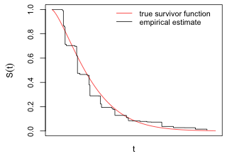
Because of its relationship to the cumulative distribution function and the fact that T has a support set that is non-negative it immediately follows that any survivor function must satisfy S(0) = 1, S(∞) = 0, and be monotone nonincreasing. Fig. 4 displays a possible survivor function along with its empirical estimate. Because we will only observe failures at discrete times, the empirical estimate of the survivor function is a step function.

Fig. 4  A survivor function along with its empirical estimate derived from a sample of survival times

The hazard function h(t) is defined to be the instantaneous potential per unit time for an event to occur in the next instant given that the individual has survived to time t. It is also called the conditional failure rate and is defined formally as follows.

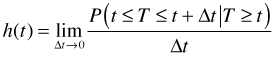
Based on the formula the hazard is the instantaneous rate per unit time of the probability of failing in the next instant of time given survival up to this point. Notice that the hazard is not a probability per se but is rather a probability rate. While the hazard function is non-negative unlike a probability the hazard can exceed one.

Just as a probability density function fully characterizes a random variable, so does the hazard function. The usefulness of the hazard function is that it is directly related to the risk of occurrence of an event over time and thus has an intuitive appeal in characterizing risk. Probability models in parametric survival analysis are typically chosen based on the behavior of their hazard functions.

1. A constant hazard is characteristic of the exponential distribution.
2. A monotone hazard, one that is always nonincreasing or always nondecreasing, is characteristic of the Weibull distribution. The exponential distribution is a special case of the Weibull.
3. A hazard that initially increases and then decreases is characteristic of the lognormal distribution.

The hazard and survivor functions are closely related and one can easily be derived from the other.

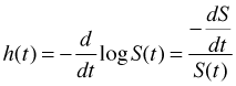
Furthermore the first of these identities implies that

The basic activities of survival analysis

1. Estimate the survivor function (or equivalently, the hazard function). The Kaplan-Meier estimate of the survivor function is the typical choice.
2. Compare the survivor functions of two or more groups. The log-rank test is the standard approach.
3. Relate the survivor function (or the hazard) to explanatory variables. This is a regression problem in which we want to relate an individual's survival history to certain exposure variables while controlling for potential confounding variables. The standard approaches here are Cox regression (a semi-parametric approach) or Weibull regression (a parametric approach).

The Kaplan-Meier estimator of the survivor function

Crucial to the development of any estimate of the survivor function is the notion of a risk set. Let denote the ordered failure times. We define the risk set as the set of individuals who have survived at least to time . Consider first a case where there is no censoring. Let n_i = number of individuals alive just before time and let m_i = the number of deaths at time . Suppose we have the following data.

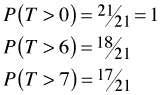
	ni	mi
0	21	0
6	21	3
7	18	1

We can easily write down the survivor function at times 0, 6, and 7. We calculate it as the number of individuals that lived past the given time divided by the number of individuals we started with.

Although it's not useful in this particular instance, we can calculate the last probability in a different way by conditioning on the previous event.

Sticking in the numbers from Table 2 yields the following.

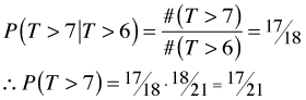
which is the same as before. Now suppose we have a censored observation at time T = 6 so that our data are as shown in Table 3. The column labeled q_i indicates the number of individual censored just after time

	ni	mi	qi
0	21	0	0
6	21	3	1
7	17	1	2

With censoring, the risk set changes and our first method of calculating the survivor function is no longer possible, but the second method will work. The first two calculations of the survivor function remain the same, but the third will be different because #(T > 6) has changed due to censoring.

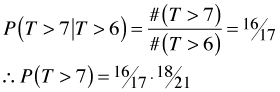
which is not the same as before. This calculation of the survival probabilities based on conditioning is the basis for the Kaplan-Meier estimator.

Course Home Page