Lecture 25—Wednesday, March 14, 2012

Topics

• Local polynomial regression (continued)
  • Kernel estimation
  • Local polynomial regression (in strictu)
  • Robustness
  • Local polynomial regression in R
• Spline models
  • Global polynomial regression
  • Polynomial splines
    • Truncated power series basis
    • B-spline basis
  • Penalized splines
  • Smoothing splines
  • Splines in R
• References

Local polynomial regression (continued)

We continue our discussion of local polynomial regression, also known as lowess. Lowess can provide a faithful local snapshot of the relationship between a response variable and a predictor. As we noted last time lowess is based on the following five ideas.

1. Binning
2. Local averaging
3. Kernel estimation
4. Local polynomial regression (in strictu)
5. Robust regression

So far we've discussed binning and local averaging.

• Binning. We use the predictor to construct a set of bins, a collection of intervals that form a partition of the x-axis. We average the values of the response variable of all observations assigned to a bin. The mean is then used as the predicted response at the x-value that corresponds to the midpoint of the bin.
• Local averaging. Local averaging is a modification of simple binning that allows observations to be used more than once. We replace the bin with a moving window that we move from observation to observation. Each time we average the observations contained in that window to obtain the predicted value of an observation. Unlike simple binning local averaging yields a prediction for each observation.

Kernel estimation

Local averaging typically yields a curve that is rather choppy as observations enter and leave the window. Furthermore while points near x₀ are indeed informative about f(x₀), they are not equally informative. We can obtain a smoother curve if we replace local averaging with locally weighted averaging, also known as kernel estimation. A kernel function is a function that weights observations that are close to the focal value x₀ more heavily than observations that are far away. If K is the kernel function then the weights at locations x_i near x₀ take the following form.

Here h is called the bandwidth. Functions typically used as kernel functions are the tricube kernel, the Gaussian kernel, and the rectangular kernel. The tricube function is defined as follows.

Each kernel function K satisfies the following properties.

With the weights calculated from the kernel we estimate f(x₀) using the n observed values of y_i as follows.

where w_i = 0 for observations whose distance from x₀ exceeds the band width. By adjusting the band width or equivalently the span, the proportion of data that are assigned nonzero weights, we can adjust the smoothness of the displayed estimate of f.

Local polynomial regression (in strictu)

To improve our estimate of f(x₀) we can take advantage of the relationship between y and x. Currently we are using the x-values only to determine the weights in the kernel function that are then used in a weighted sum of the neighboring y-values. Instead we can carry out a weighted regression of y on x for the observations contained in each window with the weight given by the kernel function. So, in each window we fit the regression equation

where typically p = 1, 2, or 3. We estimate the parameters a, b₁, … , b_p by minimizing (ordinary least squares) or by minimizing (weighted least squares). The regression equation then provides us with an estimate of f(x₀).

Robustness

While local polynomial regression yields a perfectly legitimate estimate of f, the estimate can be sensitive to outliers. To minimize the effect of outlying values most local polynomial regression routines carry out an additional step. From the local polynomial regression we obtain the estimated residual, , for each observation. Using the residual we calculate a second weight, , where W is a kernel function. Typical choices for W are the bisquare function or the Huber weight function (in which the weight is constant in a neighborhood of zero outside of which it decreases with distance). The weight function W serves as a tuning constant so that the influence of an observation on the regression model varies inversely with how far its residual is removed from zero.

We refit the local polynomial regression model but this time we minimize the objective function where w_i is the kernel neighborhood weight and W_i is the robustness weight. This whole process is then repeated. Typically two bouts of reweighting are sufficient.

Local polynomial regression in R

Local polynomial regression can be carried out in R with the lowess and loess functions of base R. These functions differ in their defaults, syntax, and the organization of their return values but otherwise they do the same thing. Additive models with loess smoothers of multiple predictors can be fit using the gam package. The syntax takes the form: y ~ gam(lo(x1) + lo(x2) + lo(x1, x2).

Spline models

Spline models are piecewise regression functions in which the pieces are constrained to connect at their endpoints (yielding a continuous curve). Usually we require that both the first and second derivatives of the resulting curve be continuous at the join points (yielding a smooth curve). A popular example of a spline model is a cubic regression spline. Although cubic regression splines tend to yield results that are nearly indistinguishable from lowess they do so using a very different approach, one that readily generalizes to more complicated regression models such as those for structured and/or correlated data.

Global polynomial regression

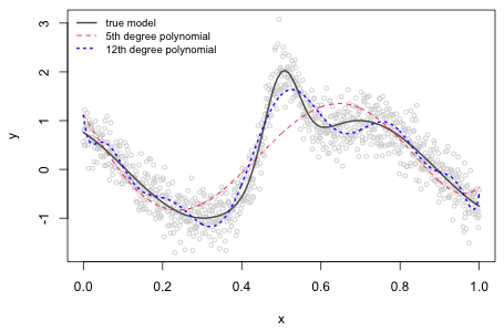
Fig. 1 displays some data values along with the nonlinear model that was used to generate them. The observations are normally distributed with a mean given by the nonlinear model and a standard deviation of 0.3. Given the complicated pattern that is shown we might consider approximating the relationship between y and x with a polynomial. The graph of the true model has four critical points (places with horizontal tangents) over the range of the data suggesting that we would need at minimum a 5th degree polynomial to duplicate this. Fig. 1 shows a 5th degree and a 12th degree polynomial that were fit to these data using least squares.

Fig. 1  Nonlinear function along with two different approximating polynomial regression models

The 5th degree polynomial has correctly detected only two of the four actual critical points and has completely missed the global maximum at x ≈ 0.5. In addition it has found a completely spurious local minimum near the right hand endpoint of the data range. The 12th degree polynomial, on the other hand, detects all four critical points but not at the correct locations. It has also introduced a number of extra wiggles and inflection points that are not seen in the true model.

Higher order polynomial regression models tend to have numerical problems. Below is just a portion of the summary table output of the 5th degree polynomial model showing the correlations of the coefficient estimates. Over half the correlations exceed 0.90 in absolute value and none of the rest are small.

The situation is even worse with the 12th degree polynomial. In addition to having highly correlated coefficient estimates, the estimates are also highly unstable. Eight of the coefficient estimates exceed 1 million (in absolute value) even though the predictor lies in the interval (0, 1) and the response variable does not exceed 3 in absolute value.

The correlation of the coefficient estimates is so severe that if we try to fit a polynomial of a higher degree, the design matrix ends up being singular and we obtain missing values for some of the coefficient estimates.

Polynomial splines

With quadratic and cubic polynomial regression models correlations between coefficient estimates can be reduced by centering the predictor. This is typically accomplished by subtracting the mean of the predictor from each observed value and then carrying out regression on the centered values. For higher order polynomial models centering doesn't work and the correlations can be severe. From a modeling standpoint the basic problem with polynomials is that they are non-local: changing a single data value affects the fit of the model over the entire range of the data. We see this in Fig. 1 where in order to constrain the polynomials to have critical values at the correct places, additional critical values and inflection points had to be introduced in places where none should exist.

A solution to the intractability of global polynomial models is to parallel what we did with lowess. Instead of fitting a single high order polynomial model to all the data simultaneously we bin the data and fit separate lower order polynomials (cubic is the typical choice) to the data in each bin. We do this in such a way that the separate pieces link up smoothly. The boundaries of the bins are referred to as knots. This raises two questions.

1. How do we choose an appropriate number of knots, and
2. how do we choose the locations of the knots?

Once we've decided on the number of knots then two popular choices are to (1) place them at equally spaced locations over the range of the predictor, or (2) place them at quantiles of the predictor. To choose the number of knots we could fit a number of spline models with different numbers of knots and choose the one that visually provides an optimal degree of smoothness. This is analogous to fitting a sequence of lowess models and varying the span (or equivalently the fraction of observations used in each window). Certain kinds of splines manage to avoid the problem of knots altogether as will be discussed later.

There are three reasons why spline models are preferred over global polynomial models.

1. The analytical foundation of spline models is superior to global polynomial models.
2. Spline models can be fit in such a way so as to prevent overfitting.
3. Spline terms can readily be combined with parametric terms to yield what are called semiparametric models.

Truncated power series (TP) basis

The easiest polynomial spline model to understand is one that uses a truncated power series basis. In linear algebra a basis for a set V is defined to be a linearly independent set of elements of V such that any element of V can be written as a linear combination of the members of the basis. A linear combination of truncated power series basis elements can be used to represent functions.

The first few elements of a truncated power series basis are the individual terms of a non-local polynomial of order l, where typically we let l = 2 or 3. For l = 2 these terms would consist of a constant term, a linear term, and a quadratic term. For l = 2 the remaining elements of the truncated power series basis would be quadratic terms, , one for each knot k_i, such that each quadratic term is identically zero for x < k_i but nonzero for x ≥ k_i. The individual quadratic terms are defined as follows.

Each represents a parabola with vertex at (k_i, 0) where we have only the right branch of the parabola.

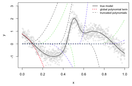
For the data in Fig. 1 suppose we choose ten equally spaced knots starting at 0.05 and ending at 0.95, each 0.10 units apart. For l = 2 a polynomial spline regression model using a TP basis would be the following.

The R code below fits this model and displays a graph of the individual terms of the TP basis scaled by their estimated γ values.

Fig. 2  Nonlinear function along with the estimated truncated power series basis terms from a quadratic polynomial spline model

If we add the global polynomial term to the individual truncated polynomials at each value of the predictor x we obtain the polynomial spline prediction of the function (Fig. 3). Observe that the fit is quite good and is better than what was obtained with the 12th degree global polynomial model we fit earlier even though 13 parameters are estimated in both cases.

Fig. 3  Nonlinear function along with the estimated quadratic polynomial spline model using a TP basis and 10 knots.

B-spline basis

While the truncated polynomial basis avoids some of the problems associated with global polynomial regression models, it can still suffer from numerical instability because the elements of the TP basis are all unbounded above. Furthermore because each polynomial is nonzero for x ≥ k_i the domains of the different terms substantially overlap with each other. Because of this the TP basis is not the ideal choice for local polynomial regression. A better choice is to use a B-spline basis.

A B-spline basis is not especially interpretable; its attraction comes from its analytical tractability. The B-spline basis can be obtained from a recurrence relation. The j^th B-spline of order l is defined as follows.

Here k_j–l, k_j, k_j+1, and k_j+1–l are knots. Notice that the order l B-spline basis is defined in terms of order l – 1 B-spline basis elements. To get things started we need an explicit expression for the order l = 0 B-spline basis.

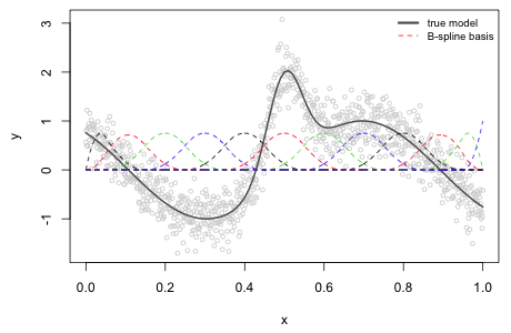
where d is the number of knots. Each of these zero order B-splines is an example of a Haar function, a kind of step function. To obtain the first order B-spline basis we use the recurrence relation on the zero order B-spline basis elements. From the formula each term will be linear in the variable x. The second order B-spline basis is also defined using the recurrence relation but this time in terms of the first order B-spline basis. Since each of the first order B-spline basis elements is multiplied by the variable x in the formula we end up with quadratic terms. Fig. 4 shows the entire second order B-spline basis for the data of Fig. 1.

Fig. 4  Nonlinear function along with the 12 elements of a quadratic B-spline basis with knots at 0.05, 0.15, … , 0.95.

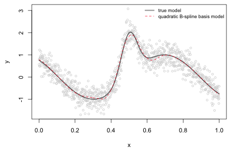
Using the second order B-spline basis as predictors in a linear regression model we can obtain the corresponding polynomial spline regression model (Fig. 5).

Fig. 5  Nonlinear function along with the estimated polynomial spline model using a quadratic B-spline basis and 10 knots.

Penalized splines

Penalized splines take a more systematic approach to the problem of knots. Consider the following more general version of the truncated power series basis that we considered earlier. This time the number and placement of the knots is left unspecified.

Written in matrix formulation this is the following.

Here X is the design matrix whose columns consist of the TP basis elements and γ is a vector of regression coefficients. The number of knots is d. Coefficient estimates can be obtained with the method of least squares by minimizing the following sum of squares.

Here are the elements of the TP basis and corresponds to the full truncated power series regression model shown above. The d terms of this expression that correspond to the truncated polynomial terms contribute a local roughness to the model to compensate for the smoothness imposed by the global polynomial portion. In matrix notation we can write the least squares solution as follows.

With penalized splines we start with a large number of knots, so many knots that we're clearly overfitting the data. In the extreme case we would choose one knot for each unique value of x but in practice this causes numerical problems and so some large subset is chosen instead. We then find γ and λ that minimize the following penalized least squares objective function.

λ is the smoothing parameter and is used to control the roughness of the polynomial spline fit. When λ = 0 the penalty term drops out and we obtain the ordinary least squares solution. For a fixed nonzero value of λ the penalty term contributes a positive amount to the objective function and the coefficients of the truncated polynomial terms have to be adjusted from their least squares values. The penalized least squares solution finds the values of γ₁, γ₂, … γ_d+3, and λ that minimize the penalized least squares criterion. With penalized splines we replace the problem of choosing the optimal number of knots with choosing an optimal value for λ.

When the TP basis is replaced with a B-spline basis the terms in the penalized least squares objective function don't neatly divide into a smooth component and a roughness component, so we need to take a more general approach. We choose the following as the penalty term.

The second derivative of a function is related to its curvature and the penalty term is the squared rate of change of the slope added up over the entire range of the estimates. So by using a penalty based on the second derivative we elect to penalize approximating functions that wiggle too much. For a function generated from a B-spline basis the second derivative can be approximated by taking second order differences of the coefficients of the B-spline basis. In general we can construct a penalized least squares criterion based on r^th order differences as follows.

where

The penalized least squares criterion can also be expressed in matrix notation.

where K is called the penalty matrix. The PLS solution for a fixed λ takes the following form.

and the spline model prediction of the vector of responses is given by

where S is called the smoothing matrix and is analogous to the hat matrix of ordinary linear regression.

It's worth noting that the PLS solution takes the same form as the solution to a regression model with random effects when the variance components are known. Consequently it is possible to represent a penalized spline model as a mixed model. We think of the data that lie between a set of knots as comprising a group and one random coefficient is assigned to each knot. In a penalized spline model the random effects are used to model the nonlinearity rather than any unobserved heterogeneity. Continuing the analogy when λ = ∞ we have the common pooling model and when λ = 0 we have the separate slopes and intercepts model.

Smoothing splines

We can generalize penalized splines even further by leaving the form of the approximating function f unspecified. This leads to the following penalized least squares criterion.

It turns out that the optimal choice for f in this expression is a special class of functions known as natural cubic splines, which are a subset of ordinary polynomial splines. A function f is a natural cubic spline with knots a ≤ k₁ < k₂ < … < k_d–1 < k_d ≤ b if

1. f is a cubic polynomial spline at the interior knots.
2. f satisfies the boundary conditions, . These boundary conditions constrains f to be linear on the intervals [a, k₂] and [ k_d–1, b].

A natural spline basis can be obtained as only a slight modification of the B-spline basis we considered earlier.

With penalized and smoothing splines we avoid the problem of choosing the number and location of the knots by replacing it with the problem of estimating a single tuning parameter λ. We use cross validation to estimate λ as follows. Fix λ at some specific value. Remove one of the observations, call it x_i. Use the remaining n – 1 observations and the formula for the penalized least squares solution given above to estimate the natural spline function. Obtain the prediction of the value of the response for the deleted observation, . Repeat this for each of the n observations and then calculate the cross validation criterion shown below.

Choose λ that minimizes this quantity.

Fortunately it's unnecessary to carry out the regression n times for a given value of λ. Instead we can estimate the smoother only once using all the data and obtain the cross validation criterion as follows.

Here is the estimate of the smoother at x_i and s_ii is the i^th diagonal element of the smoothing matrix S that was defined above. The matrix S can be difficult to calculate so the cross validation criterion is usually replaced with what's called the generalized cross validation criterion.

In the GCV we replace s_ii with the average of the diagonal elements of S. This is a savings because while calculating S may be difficult it is possible to calculate tr(S) from the component matrices of S without calculating S explicitly.

The tr(S) is referred to as the equivalent degrees of freedom and is interpreted as the effective number of parameters of a smoother. It can be used to construct an AIC measure for comparing models. For an ordinary polynomial spline model the effective number of parameters is the number of elements of the basis. For penalized and smoothing splines the effective number of parameters decreases from this value as the smoothing parameter λ is increased.

Splines in R

The functions bs and ns from the splines package of R can be used to generate a basis of B-splines and natural splines respectively that can then be used in regression models. As we've seen to use these two functions we need to specify the knot locations. There are other packages that implement penalized and smoothing splines. Two packages that permit the incorporation of a wide class of smoothing terms directly in regression models are the gam and mgcv packages. Both of these packages fit what are called generalized additive models. The gam package uses a backfitting algorithm to estimate the models while the mgcv package (acronym for multiple generalized cross validation) uses iteratively reweighted least squares and maximum likelihood.

The s function of mgcv calculates various smooths and offers an array of choices for the spline basis. All of these are penalized splines so there is no need to specify knots. On the other hand there is an argument k that is sometimes needed to specify the dimension of the basis used to represent the smooth. The default value of this parameter can occasionally be too small yielding a less than optimal smooth.

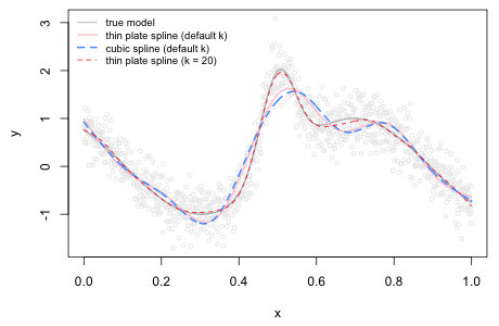
To illustrate the use of the k argument I fit a smooth to the data of Fig. 1 using the mgcv package. The default spline choice for the s function is a thin plate spline. If we specify instead a cubic spline we see that there is very little difference in the two choices (Fig. 6). Notice that neither model has tracked the true model very well. That's because the default dimension of the basis used to represent the smooth term is set too low. When we increase it by specifying k = 20 the resulting spline curve provides a closer fit to the true model.

Fig. 6  Adjusting the basis dimension of the s function of the mgcv package

References

• Fahrmeir, L., T. Kneib, S. Lang, and B. Marx. 2013. Regression: Models, Methods, and Applications. New York: Springer. Chapter 8, Nonparametric regression, 413–533.
• Keele, Luke. 2008. Semiparametric Regression for the Social Sciences. New York: Wiley.

Course Home Page