Lecture 1—Monday, January 9, 2012

Topics

• Review of simple linear regression
  • Method 1: Ordinary least squares (OLS)
  • Method 2: Linear algebra
  • The role of statistics in regression
• Multiple regression
  • Why multiple regression?

Terminology

• confounder
• interaction
• ordinary least squares
• predictor
• response variable

Review of simple linear regression

In the classic case of simple linear regression we have one continuous variable called the response, usually denoted y, and a second continuous variable called the predictor, usually denoted x. The observations consist of the ordered pairs , i = 1, 2, … , n. A scatter plot of y versus x suggests there may be a systematic relationship between the two variables (Fig. 1a). In the simplest case we look for a straight-line relationship between them, an equation of the form

where β₁ is the slope and β₀ is the intercept, and denotes the corresponding point on the regression line (also called the predicted value).

Method 1: Ordinary least squares (OLS)

The OLS solution to the linear regression problem is to find β₀ and β₁ that minimize the following quantity.

The quantity being squared is referred to as the regression error and corresponds to the vertical deviation of an observation from the regression line (Fig. 1b). The entire quantity that is minimized is called the sum of squared errors (SSE).

(a)	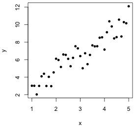(b)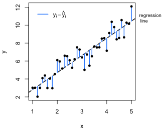
Fig. 1 (a) Scatter plot of y versus x suggesting a linear relationship. (b) The OLS regression line minimizes the sum of the squared vertical deviations from the regression line,

This problem is easily solved using calculus. To do so we obtain two derivatives, the derivative of SSE with respect to β₀ and the derivative of SSE with respect to β₁, set both derivatives equal to zero, and solve simultaneously for the parameters β₀ and β₁. We write the solution as follows.

where we place carets over the parameter symbols to indicate that these are the values that were estimated from the data using OLS.

Ordinary least squares is just one way of constructing a "best-fitting" line to a scatter plot of data. Other methods include the following.

1. Instead of minimizing the sum of the squared vertical deviations we could minimize the sum of the absolute values of the vertical deviations, . This yields the L₁-norm solution to the regression problem.
2. Rather than minimizing the sum of squared vertical distances from the line we could use squared perpendicular (shortest) distances. This yields what's called the major axis (MA) regression solution.
3. We could use each point to construct a right triangle: one leg of the triangle is the vertical deviation of the point from the line, the second leg of the triangle is the point's horizontal deviation from the line, and the hypotenuse of the triangle consists of the line itself. We could then minimize the sum of the areas of all the little triangles we create. This is called reduced major axis (RMA) regression.

The second and third methods listed above are sometimes referred to as Type II regressions, whereas OLS is referred to as Type I regression. Historically the OLS solution has been preferred because it was considered simpler to compute and has nice properties.

Method 2: Linear algebra

The regression problem of fitting a line to a 2-dimensional scatter plot of data can also be treated as a problem in n-dimensional geometry. The n observed values of the response variable define an n × 1 vector y and the corresponding n values of the predictor define an n × 1 vector x. The regression equation relates these two vectors in a matrix equation as follows.

The matrix X is referred to as the design matrix of the system. Row-reducing the augmented matrix [X|y] to find a solution to this matrix equation is futile here. Linear algebra theory tells us that an n × 2 system of equations, where n > 2, typically corresponds to an inconsistent system of equations and will not have a solution. Of course we already knew this because we've seen that the points don't all lie on a single straight line (Fig. 1a).

The matrix product Xβ can be interpreted as taking a linear combination of the columns of the matrix X using coefficients that are the components of β.

The vectors y, 1, and x in the above equation can be visualized as three vectors in n-dimensional space (Fig. 2). The vectors 1 and x define a plane in n-dimensional space (as do any two non-collinear vectors) and by specifying values for β₀ and β₁ in the above linear combination we obtain different points in that plane. As Fig. 2 shows, the vector y will typically not lie in the plane defined by the vectors 1 and x. For that reason the matrix equation fails to have a solution. The vector y cannot be written as a linear combination of the vectors 1 and x.

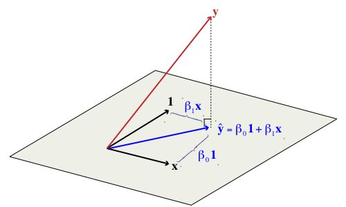
Fig. 2  The regression problem viewed as vector projection in n-dimensional space

We can salvage a solution to this problem as follows. Find the vector that lies in the plane defined by the vectors 1 and x such that its distance from the vector y is shortest. Geometrically we can obtain by dropping a perpendicular from y onto the plane defined by 1 and x. Algebraically we do this by projecting the vector y onto this plane, a feat that is accomplished by premultiplying y by an appropriate projection matrix. The components of the coefficient vector β are obtained as follows.

and the projected vector is given by

where is the desired projection matrix.

Interestingly this solution obtained using projection matrices is identical to the ordinary least squares (OLS) solution. So, we get the same answer to the regression problem regardless of whether we view it as a calculus minimization problem or a vector projection problem. Either way finding the coefficients of the regression equation is a straight-forward mathematical problem with a well-defined solution.

The role of statistics in regression

Everything we've done so far is just mathematics. So, where does statistics enter the picture? Mathematics gives us a line that best fits the data, where we define "best" in a way that suits us. If the data were obtained as a sample from a population then the equation fit to that specific data set is probably not that interesting by itself. It is the corresponding regression equation in the sampled population that we truly care about. The target population may be real (as when we have a list of potential observations and we've obtained only a subset of them) or more hypothetical (e.g., the set of all possible ways we might lay out a set of quadrats in a field and then count the number of individuals of a particular species in each quadrat).

What we want to be able to say is that the regression equation we obtained using our data set also represents the regression equation in the population. The concern we should have with estimating a regression equation based on a sample is that if we were to go back and collect data a second time the sample we would obtain would be different and produce a different regression equation. Because we know a sample-derived regression equation will vary from sample to sample we need to quantify how much it is likely to vary and include this information in our report.

Based on a single sample what can we say about the population that gave rise to it? Surprisingly, quite a lot. We don't actually have to go back and get additional samples.

1. If our sample is a random (or at least a probabilistic) sample from the population, then there is standard statistical theory that tells us how much the statistics we calculate using that sample are likely to vary if we were able to obtain multiple samples from the same population. For instance, statistical theory tells us that the sample mean based on a sample of size n has a variance of

where σ² can be estimated from s², the variance of the sample data.

2. If we can assume that the response variable y is normally distributed, statistical theory tells us that the OLS solutions and are also normally distributed. The means of these normal distributions equal the corresponding population values and their variances can be estimated directly from the least squares fit.
3. If the response variable y is not normally distributed then the least squares solutions are not necessarily normally distributed. It turns out in this case that if we use maximum likelihood estimation instead of OLS, the regression coefficients will again be normally distributed regardless of the distribution of y. We'll discuss this approach to estimation beginning in week 3 of this course.

The OLS solution yields the best-fitting line to a data set, but to go further and draw inferences about the population from which the data were obtained we generally need to make additional assumptions about the sample and the population. The regression equation is then used to characterize a particular parameter in the distribution of the response variable y, often the mean of that distribution.

Multiple regression

Multiple regression differs from simple linear regression in that we have multiple predictor variables. Mathematically multiple regression is just a trivial extension of the simple linear regression problem. The methods of solution that worked for simple linear regression also work for multiple regression. For example, if the multiple regression problem has three predictors x, z, and w so that the regression equation is

we can find the least squares solution by constructing the sum of squares error as before

The only difference is that now instead of two partial derivatives there are four partial derivatives to calculate and set equal to zero. From a linear algebra perspective the difference between simple and multiple regression is even more trivial. In multiple regression the design matrix X just has more columns in it.

The solution is found in the same way as before, .

It's worth noting that the thing that makes linear regression "linear" is the fact that the regression equations can be written in terms of matrix multiplication. This means that fitting curves such as polynomials to a data set is still a linear regression problem even though the curve we obtain isn't a line. Suppose we wish to fit a parabola to a scatter plot of y versus x.

This is still a problem in linear regression because the regression equation can be expressed in matrix form as follows.

Having powers or functions of predictors in a regression equation poses no new problems. The equation is still linear. If the regression equation can be written as a matrix product of a data matrix times a vector of parameters, it's a linear equation.

Why multiple regression?

Why is multiple regression generally preferable to simple linear regression?

1. We expect ecological and environmental processes to respond to multiple inputs. Although technically regression explores correlative relations, not causal ones, if theory suggests that there are multiple potential causative agents of a response, it makes sense to include these different agents as predictors in a regression equation. In a formal experiment it is always a more efficient use of resources to run the experiment with multiple factors affecting the response than to run separate experiments for each factor of interest. So, here again multiple regression is the preferred method of analysis.
2. When there is only a single predictor in the regression model it is possible to misinterpret that predictor's true relationship with the response. If additional variables are added as predictors in this regression equation, we may discover that the relationship between the response and the original targeted predictor is now quite different from what it was with just the targeted predictor alone. When this happens the additional predictors are referred to as confounding variables. Controlling for confounding is one of the primary uses of multiple regression.
3. Including two or more variables in a regression equation allows us to investigate the phenomenon of interaction. If the predictors x and z interact it means that the relationship between y and x is different for different values of z. This may sound like confounding but it isn't. With confounding the relationship between y and x doesn't change according to the value of z. It stays the same for each different value of z but it is different from what it was when we ignored the existence of z altogether. Generally speaking, if we find that the predictors x and z interact then the notion of confounding is not applicable. Therefore the usual protocol is to first check for interaction and then check for confounding only if interaction is absent.

We'll explore the concepts of confounding and interaction further in lecture 2.

Course Home Page